Service workload patterns for Qos-driven cloud resource management

Abstract

Cloud service providers negotiate SLAs for customer services they offer based on the reliability of performance and availability of their lower-level platform infrastructure. While availability management is more mature, performance management is less reliable. In order to support a continuous approach that supports the initial static infrastructure configuration as well as dynamic reconfiguration and auto-scaling, an accurate and efficient solution is required. We propose a prediction technique that combines a workload pattern mining approach with a traditional collaborative filtering solution to meet the accuracy and efficiency requirements. Service workload patterns abstract common infrastructure workloads from monitoring logs and act as a part of a first-stage high-performant configuration mechanism before more complex traditional methods are considered. This enhances current reactive rule-based scalability approaches and basic prediction techniques by a hybrid prediction solution. Uncertainty and noise are additional challenges that emerge in multi-layered, often federated cloud architectures. We specifically add log smoothing combined with a fuzzy logic approach to make the prediction solution more robust in the context of these challenges.

Introduction

Quality of Service (QoS) is the basis of cloud service and resource configuration management [1, 2]. Cloud service providers – whether at infrastructure, platform or software level – provide quality guarantees usually in terms of availability and performance to their customers in the form of service-level agreements (SLAs) [3]. Internally, the respective service configuration in terms of available resources then needs to make sure that the SLA obligations are met [4]. To facilitate SLA conformance, virtual machines (VMs) can be configured and scaled up/down in terms of CPU cores and memory, deployed with storage and network capabilities. Some current cloud infrastructure solutions allow users to define rules manually to scale up or down to maintain performance levels.

QoS factors like service performance in terms of response time or availability may vary depending on network, service execution environment and user requirements, making it hard for providers to choose an initial configuration and scale this up/down to maintain the SLA guarantees, but also optimising resource utilisation at the same time. We utilise QoS prediction techniques here, but rather than bottom-up predicting QoS from monitored infrastructure metrics [5–7], we reverse the idea, resulting in a novel technique for pattern-based resource configuration.

A pattern technique is at the core of the solution. Various types of cloud computing patterns exist [8], covering workload, but also offer types and application and management architectures. These patterns link infrastructure workloads such as CPU utilisation with service-level performance. Recurring workloads have already been captured as patterns in the literature [8], but we additionally link these to service quality.

We determine service workload patterns through pattern mining from resource utilisation logs. These service workload patterns (SWPs) correspond to typical workloads of the infrastructure and map these to QoS values at the service level. A pattern consists of a relatively narrow range of metrics measured for each infrastructure concern such as compute, memory/storage and network under which the QoS concern is stable. This can be best illustrated through utilisation rates. Should resources be utilised in a certain range, e.g., low utilisation of a CPU around 20 %, then the response-time performance can be expected to be high and not impacted negatively by the infrastructure.

These patterns can then be used in the following way. In a top-down approach, we take a QoS requirement and determine suitable workload-oriented configurations that maintain required values. Furthermore, we enhance this with a cost-based selection function, applicable if many candidate configurations emerge.

We specifically look at performance as the QoS concern here since dealing with availability in cloud environments is considered as easier to achieve, but performance is currently neglected in practice due to less mature resource management techniques [4]. We introduce pattern mining mechanisms and, based on a QoS-SWP matrix, we define SWP workload configurations for required QoS. The accuracy of the solution to guarantee that the chosen (initially predicted) resource configurations meet the QoS requirements is of utmost importance. An appropriate scaling approach is required in order to allow this to be utilised in dynamic environments. In this paper, we show that the pattern-based approach improves the efficiency of the solution in comparison with traditional prediction approaches, e.g., based on collaborative filtering. This enhances existing solutions by automating current manual rule-based reactive scalability mechanisms and also advances prediction approaches for QoS, making them applicable in the cloud with its accuracy and performance requirements.

Cloud systems are typically multi-layer architectures with services being provided at infrastructure, platform or software application level. Uncertainty and noise are additional challenges that emerge in these multi-layered, often federated clouds architectures. We extend earlier work [9] to address these challenges. We propose to use log smoothing and a fuzzy logic-based approach to make the prediction solution more robust in the context of these challenges. Smoothing will deal with log data variability and will allow detecting trends (but adds more noise). Uncertainty often occurs as to the completeness and reliability of monitored data, which will here be addressed through a fuzzy logic enhanced prediction. We will demonstrate the robustness of the solution against noise and uncertainty.

Section ‘Quality-driven configuration and scaling’ outlines the solution and justifies its practical relevance. Section ‘Workload patterns’ introduces SWPs and how they can be derived. Section ‘Quality pattern-driven configuration determination’ discusses the selection of patterns as workload specifications for resource configuration. The application of the solution for SLA-compliant cloud resource configuration is described in Section ‘Pattern-driven resource configuration’. Section ‘Managing uncertainty’ deals with uncertainty through a fuzzification of the patterns. Section ‘Evaluation’ contains an evaluation in terms of accuracy, performance and robustness of the solution and Section ‘Related work’ discusses related work.

Quality-driven configuration and scaling

Cloud resource configuration is the key problem we address. We start with a brief discussion of the state-of-the-art and relevant background.

An SLA is typically defined based on availability. Customers expect that the services they acquire will be always available. Thus, providers usually make clear and reliable claims here. The consensus in the industry is that cloud computing providers generally have solutions to manage availability. Response time guarantees, on the other hand, are harder to guarantee [4]. These types of obligations are more carefully phrased or fully ignored. A quote to illustrate this is “We are putting a lot of thought into how we can offer predictable, reliable and specific performance metrics to a customer that we can then [build an] SLA around,” [C. Drumgoole, vice president global operations, Verizon Terremark, 2013]. Thus, we specifically focus on performance, although our solution is in principle applicable to availability as well. From a providers perspective, the question is how to initially configure and later scale VMs and other resources for a service such that the QoS (specifically response time) is guaranteed and, if additionally possible, cost is optimised. From an infrastructure perspective, memory, storage, network conditions and CPU utilisation impact on QoS such as performance and availability significantly. We consider data storage size, network throughput and CPU utilization as representatives of data, network and computation characteristics. Common definitions, e.g., throughput as the rate of successful message delivery over a communication channel or bandwidth, shall be assumed. Figure 1 illustrates in a simple example that values of the three resource configuration factors can be linked to the respective measured performance. It shows how the performance differs depending on the infrastructure parameters, but not necessarily in a way that would be easy to determine and predict.

Fig. 1

Measured QoS mappings: Infrastructure to Servic ([CPU, network, storage] → Performance)

The first step is to monitor and record these input metrics in system-level resource utilisation logs. The second step is pattern extraction. From repeated service invocations records (the logs), an association to service QoS values based on prediction techniques can be made. An observation based on experiments that we made is that most services have relatively fixed service workload patterns (SWP):

• The patterns are defined here as ranges of storage, network and CPU processing characteristics that reflect stable, small acceptable variations of a QoS value.

• Generally, service QoS keeps steady under a SWP, allowing this stable mapping between infrastructure input and QoS to be used further.

If we can extract SWPs from service logs or the respective resource usage logs (based on pattern mining), the associated service quality can be based on usage information using pattern matching and prediction techniques. Even if there is no or insufficient usage information for a given service, quality values can be calculated using log information of other similar services, e.g., through collaborative filtering. These two steps can be carried out offline. The next, first online step is pattern matching, where dynamically a pattern is matched in the matrix against performance requirements. The final step is the (if necessary dynamic) configuration of the infrastructure in the cloud.

The hypothesis behind our workload pattern-driven resource configuration based on required service-level quality is the stability of variations of quality under SWPs. We assume SLA definitions to establish QoS requirements and the charged costs for a service to be decided between provider and consumer. Service-specific workload pattern are mined and constructed which considers environmental characteristics of a service (in a VM) deployment. We experimentally demonstrate that the hybrid technique for QoS-to-SWP mappings (based on pattern matching and collaborative filtering for missing information) enhances accuracy and computational performance and makes it applicable in the cloud. In contrast, traditional prediction techniques can be computationally expensive and unsuitable for the cloud.

We limit this investigation to services and infrastructure with some reasonably deterministic behaviour, e.g., classical business or technology management applications. However, we deal with larger substantial uncertainties arising from the infrastructure and platform environment in which the services are executed. We also focus on the variability of log data, noise that occurs and uncertainties arising from multi-cloud environments.

Workload patterns

The core concept of our solution is a Service Workload Pattern (SWP). A SWP is a group of service invocation characteristics reflected by the utilised resources. In a SWP, the value of workload characteristics is a range. The QoS is meant to be steady under a SWP. We describe a SWP M as a triple of ranges low to high (as l o w∼h i g h ranges):

$$ \begin{array}{ll} M=& ~ \left[~CPU_{low} \sim CPU_{high},\right.\\ &\left. ~~~Storage_{low} \sim Storage_{high},\right.\\ & \left.~~~Network_{low} \sim Network_{high} ~\right] \end{array} $$

((1))

CPU, Storage and Network are common server computation, memory and network characteristics that we have chosen for this investigation [7]. The CPU time used and utilisation rates are typically the most influential factor. The RAM (memory) utilisation rate and storage access are equally important. In distributed applications, network parameters such as bandwidth, latency and throughput have an influence of service QoS (we consider here the latter). Note that in principle, the specific characteristics could be varied.

We initially work with monitored absolute figures for CPU time used, stored data size and network throughput. Later on, we also convert this into normalised utilisation rates with respect to the allocated resources.

SWP pattern mining and construction

We assume service-level execution quality logs in the format <q ₁,…,q _n > and infrastructure-level resource monitoring logs $< {r_{1}^{i}}, \ldots, {r_{m}^{i}} >$ with i=1,…,j for j different quality aspects (e.g., storage, network, server CPU utilisation) of the past invocations of the services under consideration, as illustrated in Fig. 1. For each service, the resource metrics and the associated measured performance are recorded. The challenge is now to determine or mine combinations of value ranges for input parameters r that result in stable, i.e., only slightly varying performances. The solution is a SWP extraction process that constructs the workload patterns.

• A SWP is composed of storage, network and computation characteristics. For these, we take throughput, data size and CPU utilization as representatives, respectively.

• We consider the execution (response) time as the representative of QoS here.

An execution log records the input data size and execution QoS; a monitoring log records the network status and Web server status. We reorganize these two logs to find the SWP under which QoS keeps steady. Our SWP mining algorithm is based on a generic algorithm type, DBSCAN (density-based spatial clustering of applications with noise). DBSCAN [10] analyses the density of data and allocates the data into a cluster if the spatial density is greater than a threshold. The DBSCAN algorithm has two parameters: the threshold ε and the minimum number of points MinPts. Two points can be in the same cluster if their distance is less than ε. The minimum number of points is also given. We also need a parameter MaxTimeRange, the max time range of a cluster. We expect the range of time is a cluster that can be steady and that has a size limit. When the cluster is too large, e.g., if the range exceeds a threshold, the cluster construction should be stopped. The main steps are given in the following Algorithm 1:

• Select any object p from the object set S and find the objects set D in which the object is density-reachable from object p with respect to ε and MinPts.

• Choose another object without cluster and repeat the first step

The pattern extraction algorithm is presented in Algorithm 1.

We give higher precedence to more recent log entries. Exponential smoothing can be applied to any discrete set of sequential observations x _i . Let the sequence of observations begin at time t=0, then simple exponential smoothing is defined as follows:

$$ \begin{array}{ll} &y_{0}=x_{0}\\ & y_{t}= \alpha x_{t}+(1-\alpha)y_{t-1},t>0,0<\alpha<1 \end{array} $$

((2))

The choice of α is important. Close to 1 has no smoothing effect and gives higher weight to recent changes and as a result the estimate may fluctuate dramatically. Values of α closer to 0 have a better smoothing effect and the estimate is less responsive to recent changes. We can choose a value like 0.8 as the default, which is relatively high, but reflects the most recent multi-tenancy situation (which can undergo short-term changes). We will discuss this separately later in more detail in Section ‘Variability and smoothing’.

Pattern-quality matrix

The input value ranges form a pattern that is linked to the stable performance ranges in a Quality Matrix MS(M,S) based on patterns M and services S. MS associates a service quality Q o S P(S _i ,M _i ) (with P standing for performance) of service S _i in S under a pattern M _j in M.

$$\begin{array}{*{20}l} &\!\:\!\qquad\qquad\qquad\,\,\,\, S_{1}\quad\, S_{2}\,\,\,\,\, \ldots \quad\! S_{m}\\ &{MS} = \begin{array}{cc} &M_{1}\\ &M_{2}\\ &\ldots\\ &M_{l} \end{array}\left(\begin{array}{cccc} q_{1,1} &\,\, q_{1,2} &\,\, \ldots &\,\, q_{1,m}\\ q_{2,1} &\,\, q_{2,2} &\,\, \ldots &\,\, q_{2,m}\\ \ldots &\,\, \ldots &\,\,\ldots &\,\, \ldots \\ q_{l,1} &\,\, q_{l,2} &\,\, \dots &\,\, q_{l,m} \end{array} \right) \end{array} $$

((3))

Figure 1 at the beginning illustrated monitoring and execution logs that capture low-level metrics (CPU, storage, network) and the related service response time performance. SWPs M _i then result from the log mining process using clustering.

The following is a set of patterns M ₁ to M ₃ for the given example in Fig. 1:

$$ \begin{array}{lccc} ~ & CPU & Strg & Netw \\ M_{1} = & [\!2.1 \sim 2.5~~, & 10 \sim 11~~,& 0.1 \sim 0.2 ] \\ M_{2} = & [\! 2.0 \sim 2.2~~, & 8 \sim 30~~, & 0.2 \sim 0.4 ] \\ M_{3} = & [\! 1.2 \sim 2.0~~, & 10 \sim 20~~, & 0.1 \sim 0.5 ] \end{array} $$

((4))

For those patterns, we can construct the following quality matrix MS:

$$\begin{array}{*{20}l} &\qquad\qquad\,\,\, S_{1}\qquad\qquad S_{2}\qquad\qquad S_{3}\\ &\begin{array}{c} M_{1}\\ M_{2}\\ M_{3} \end{array} \left(\begin{array}{cccc} 0.2 \sim 0.5s &\,\, &\,\, 1.5 \sim 1.8s\\ 1.4 \sim 1.8s &\,\, 1.1 \sim 1.5s &\\ 1.5 \sim 2.1s &\,\, & \end{array} \right) \end{array} $$

((5))

The matrix MS above shows the QoS in this example for performance information of all services s _j for all patterns M _i . The quality q _ij (1≤j≤l,1≤i≤m) is the quality of service s _j under pattern M _i with the quality value q _ij defined as follows:

• as ϕ if the service s _j has no invocation history under pattern m _i and

• as l o w _ij ∼h i g h _ij if the service s _j has an invocation history under m _i with range ∼.

For a pattern M ₁=[ 0.5∼0.6,0.2∼0.4,30∼40] the CPU utilization rate is 0.5–0.6, storage utilization is 0.2–0.4 and network throughput is 30– 40 M B. The sample matrix illustrates the workload pattern to QoS association for services. Empty spaces (undetermined null values) for a service indicate lacking data. In that case, a prediction based on similar services is necessary, for which we use collaborative filtering.

Pattern matching

For monitored resource metrics (CPU, storage, network), we need to determine which of these influences performance the most. This determines the matched pattern. Let the usage information of service s be a sequence x _k of data storage D, network throughput N and CPU utilisation C values mapped to response time R for k=1,…,n:

$$ \begin{array}{ll} &\left[<{x_{D}^{1}},{x_{N}^{1}},{x_{C}^{1}}>,{x_{R}^{1}}\right]\\ & \ldots \\ & \left[<{x_{D}^{k}},{x_{N}^{k}},{x_{C}^{k}}>,{x_{R}^{k}}\right] \\ & \ldots \\ & \left[<{x_{D}^{n}},{x_{N}^{n}},{x_{C}^{n}}>,{x_{R}^{n}}\right] \end{array} $$

((6))

We use response time performance in the log as the reference sequence x _R (k),k=1,…,n, and other configuration metrics as comparative sequences. Then, we calculate the association degree of other characteristics with response time and use characteristics of an invocation as standard and carry out a normalization of the other metrics. Thus, the normalized usage information y is (schematically) for any invocation k:

$$ \left[ <y_{D}\left({x_{D}^{k}}\right),y_{N}\left({x_{N}^{k}}\right),y_{C}\left({x_{C}^{k}}\right)>, 1 \right] $$

((7))

Response time is the reference sequence x ₀(k),k=1,…,n and the other infrastructure characteristics are the comparative sequences. We calculate the associate degree of the other three characteristics with response time. We take one invocation as standard and then normalise the others. The reference (i=0) and comparison sequences (i=1,…,3) are handled dimensionless. We obtain standardised sequences y _i (k),i=0,1,…,3;k=1,…,n, see Fig. 2.

Fig. 2

Normalised QoS mappings: Infrastructure to Service ([CPU, network, storage] → Performance)

Next, we calculate absolute differences for the table above using

$$ \Delta_{oi}=|y_{o}(k)-y_{i}(k)| $$

((8))

With O _i here ranging over the quality aspects, we get O ₁=D, O ₂=N and O ₃=C. The resulting absolute difference sequence is for our 3 quality aspects the following:

$$ \begin{array}{ll} &\Delta_{01}=(0,y_{01}(1), \ldots,y_{01}(n)),\\ &\Delta_{02}=(0,y_{01}(2), \ldots,y_{02}(n)),\\ &\Delta_{03}=(0,y_{01}(3), \ldots,y_{03}(n)),\\ \end{array} $$

((9))

In the next step, we determine a correlation coefficient between reference and comparative sequence (using here the correlation coefficient of the Gray relevance):

$$ \zeta_{oi}(k)=\frac{\Delta_{min}+\rho \Delta_{max}}{\Delta_{oi}(k)+\rho \Delta_{max}} $$

((10))

Here Δ _oi (k)=|y ₀(k)−y _i k| is the absolute difference, Δ _min =m i n _i m i n _k Δ _0i (k) is the minimum difference between two poles, Δ _max =m a x _i m a x _k Δ _0i (k) is the maximum difference, ρ∈(0,1) is a distinguishing factor. Afterwards, we use the formula

$$ r_{oi}=\frac{1}{n} \sum_{i=1}^{n} \zeta_{o1}(k) $$

((11))

to calculate the correlation degree between the metrics. Then, we sort the metrics based on the correlation degree. If r ₀ is the largest, it has the greatest impact on response time and will be matched prior to others in the pattern matching process.

Clouds are shared multi-user environments where users and applications require different quality settings. A multi-valued utility function $\widetilde {U}$ can be added representing the user weighting of a vector $\widetilde {Q}$ of quality attributes q∈Q for a matrix m _i ∈M as a weighting. This utility function allows a user to customise the matching with user-specific weightings:

$$ \widetilde{U}_{\text{\textit{p,m,q}}}:rng(\widetilde{Q}_{m,q}) \rightarrow [\!0,1] $$

((12))

The overall utility can be defined, taking into account the importance or severity of the quality attributes ω _i for each q∈Q :

$$ \begin{array}{ll} &\widetilde{U}_{m} = \sum\limits_{\forall q_{i} \in Q} \omega_{i} \widetilde{U}_{m,q_{i}}\left(\widetilde{Q}_{m,q_{i}}(MS)\right)\\ &\widetilde{U}_{m,q}= \sum\limits_{\forall p \in p} \widetilde{U}_{\text{\textit{p,m,q}}}\\ &\sum\limits_{i} \omega_{i}=1,\omega_{i} \geq 0\\ \end{array} $$

((13))

Finally, the pattern that optimizes the overall configuration utility is determined through the maximum utility calculated as:

$$ {max}_{{m\in M}_{s}}\widetilde{U}_{m} $$

((14))

Note, that the utility is based on the three quality concerns, but could potentially be extended to take other factors into account. Furthermore, costs for the infrastructure can also be taken into account to determine the best configuration. We will define an additional cost function in the cloud configuration Section ‘Pattern-driven resource configuration’ below.

Quality pattern-driven configuration determination

The QoS-SWP matrix is the tool to determine SLA requirements-compliant SWPs as workload specifications for the resource configuration and re-configuration and re-scaling. For quality-driven configuration, the question is: for a given service S _i and a given performance requirement Q o S _P , what are suitable SWPs to configure the execution environment? The execution environment is assumed to be a VM image configuration with storage and network services samples are discussed in Section ‘Pattern-driven resource configuration’. We first determine a few configuration determination use cases to get a comprehensive picture where the pattern technique can be used and then discuss the core solutions in turn.

Use cases

In general, there is a possibly empty set of patterns M S(s _i ) for each service s _i , i.e., some services have usage information, others have no usage information in the matrix itself. Consider the sample matrix from the previous section. Three use cases emerge that indicate how the matrix can be used:

• Configuration Determination — Existing Patterns: For a service s with monitoring history: Since s1 has an invocation history for various patterns for a requested response time of 0.45s, we can return this set of patterns including M ₁ and M ₃.

• Configuration Determination — Non-existing Patterns: For a given service s without history: Since s ₂ has no invocation history for a required response time of 2s, we can utilise collaborative filtering for the prediction of settings, i.e., use similar services to determine patterns for the given service [11, 12].

• Configuration Test — For a given triple of SWP values and a service s: If a given s ₁ has an invocation history for a required response time of 2s and we have a given workload configuration, we can test the compliance of the configuration with a pattern using the matrix.

Pattern-based configuration determination

If patterns exist that satisfy the performance requirements, then these are returned as candidate configurations. In the next step, a cost-oriented ranking of these can be done. We use quality level to cost mappings that will be explained in Section ‘Pattern-driven resource configuration’ below. If no patterns exist for a particular service (which reflects the second use case above), then these can be determined by prediction through collaborative filtering, see [7].

QoS prediction process For any service s, if there is information of s _v under pattern mi, then calculate the similarity between other services s _j and s _v . We can get the k neighbouring services of service s _j through a similarity calculation. The set of these k services is $S = {s_{1}^{\prime },s_{2}^{\prime },\ldots,s_{k}^{\prime }}$. We fill the null (empty) QoS values for the target invocation using the information in this set. Using the information in S, we then calculate the similarity of m _i with other patterns that have the information for target service s _j . We choose the most similar k ^′ patterns of m _i , and use the information across the k ^′ patterns and S to predict the quality of service s _j .

Service similarity computation If there is no information of s _j in a pattern M _i , we need to predict the response time q _i,j for s _j . Firstly, we calculate the similarity of sj and services which have information within pattern M _i ranges. For a service s _v in I _i where I _i is the set of services that have usage information within pattern M _i we calculate the similarity of s _j and s _v . We need to consider the impact of configuration environment differences, i.e., redefine common similarity definitions. M _vj is the set of workload patterns which have the usage information of services s _v and s _j .

$$ \begin{array}{ll} & n{S}\left(s_{v},s_{j}\right)=\\ &\frac{\sum_{m_{c}} \in\, M_{vjj}\left(q_{c,v}-\overline{q_{v}}\right)\left(q_{c,j}-\overline{q_{j}}\right)}{\sqrt{\sum_{m_{c} \in\, Mvj}\left(q_{c,v}- \overline{q_{v}}\right)^{2}} \sqrt{\sum_{m_{c} \in\, Mvj}(q_{c,j}- \overline{q_{j}})^{2} }} \end{array} $$

((15))

Here, $\overline {q_{v}}$ is the average quality value for service s _v and $\overline {q_{j}}$ is the respective value for s _j . From this, we can obtain all similarities between s _j and others services which have usage information within pattern m _i . The more similar the service is to s _j , the more valuable its data is.

Predicting missing data Missing or unreliable data can have a negative impact on prediction accuracy. In [13], we considered noise up to 10 % to be acceptable. In order to deal with uncertainty beyond this, we calculate the similarity between two services and get the k neighbouring services. Then, we establish the k-neighbour matrix N _sim , see Eq. (16), and complete the missing data. N _sim shows the usage information of the k neighbour services of s _j under all patterns, reducing the data space to k columns.

$$\begin{array}{*{20}l} &\!\qquad\qquad\qquad\,\,\, s_{j}\quad\,\,\, s_{1}^{\prime}\,\,\,\,\,\: \dots\quad\, s_{k}^{\prime}\\ &N_{sim} =\begin{array}{cc} M_{1}\\ \dots\\ M_{i}\\ \dots\\ M_{l} \end{array} \left(\begin{array}{cccc} s_{1j} &\,\,\, s_{1,1} &\,\,\, \dots &\,\,\,s_{1,m}\\ \dots &\,\,\, \dots &\,\,\,\dots &\,\,\, \dots\\ s_{i,j} &\,\,\, s_{i,1} &\,\,\, \dots &\,\,\, s_{i,m}\\ \dots &\,\,\, \dots &\,\,\,\dots &\,\,\, \dots\\ s_{l,j} &\,\,\, s_{l,1} &\,\,\, \dots &\,\,\, s_{l,m} \end{array} \right) \end{array} $$

((16))

Empty spaces are filled, if required. Then, we add s _i,p as the data of service s _p under pattern m _i :

$$ \begin{array}{ll} s_{i,p}=\overline{q_{p}^{\prime}}+\frac{\sum_{n \in S^{\prime}}sim_{n,p} \times \left({q_{i,n}^{\prime}}-\overline{q_{n}^{\prime}}\right)}{\sum_{n \in S^{\prime}}(|sim_{n,p}|)} \end{array} $$

((17))

Again, $\overline {q_{p}^{\prime }}$ is the average quality value of s _p , and s i m _n,p is the similarity between s _n and s _p . Now every service s∈S ^′ has usage information within all pattern ranges in m _i .

Calculating pattern similarity and prediction There is QoS information of k neighbouring services of s _j in matrix N _sim . Some of them are prediction values. We can calculate the similarity of pattern m _i and other patterns using the correction cosine similarity method:

$$ \begin{array}{ll} &sim_{M}(m_{i},m_{j})=\\ &\frac{\sum_{s_{k}\in S} \left(t_{i,k}^{\prime}-\overline{t_{i}^{\prime}}\right)\left(t_{j,k}^{\prime}-\overline{t_{j}^{\prime}}\right)}{\sqrt{\sum_{s_{k} \in S}\left(t_{i,k}^{\prime}- \overline{t_{i}^{\prime}}\right)^{2}} \sqrt{\sum_{s_{k} \in S}\left(t_{j,k}^{\prime}- \overline{t_{j}^{\prime}}\right)^{2} }} \end{array} $$

((18))

After determining the pattern similarity, the data of patterns with low similarity are removed from N _sim , the set of the first k patterns. The data of these patterns are retained for prediction. If p _i,j is the data to be predicted as the usage data of service s _j within pattern m _i , it can be calculated.

$$ \begin{array}{ll} p_{i,j}=\overline{q_{i}^{\prime}}+\frac{\sum_{n \in M^{\prime}}sim_{n,i} \times \left({q_{n,j}^{\prime}}-\overline{q_{n}^{\prime}}\right)}{\sum_{n \in M^{\prime}}(|n{n,i}|)} \end{array} $$

((19))

The average QoS of data related to pattern m _i is $\overline {q_{i}^{\prime }}$ and s i m _n,j is the similarity between patterns m _n and m _p .

Pattern-based configuration testing

We can use the pattern-QoS matrix to test a standard or any known resource configuration in SWP format (i.e., three concrete values rather than value ranges for the infrastructure aspects) for instance in the situation outlined above for a service s _i for which its performance is uncertain. This can also be done instead of collaborative filtering, as indicated above, if the returned set of patterns is empty and a candidate configuration is available. Then, the matrix can be used to determine the respective QoS values, i.e., to predict quality such as performance in our case through testing as well.

This situation shall be supported by an algorithm that matches candidate configurations with stored workload patterns based on their expected service quality. The algorithm takes into account whether or not possibly matching workload patterns exist.

If no patterns exist, existing candidate configurations can be tested – to enable always a solution, at least one default configuration should be provided. Alternatively, similar services can be considered; these can be determined through collaborative filtering and then we would start again.

Variability and smoothing

While the solution above extracts patterns for a given log, some practical considerations shall be taken into account. In log data corresponding to resource workload measurements, we can usually observe high variations over time, which makes predictions over particularly small time-scales unreliable. The workload contains often many short-duration spikes. In order to alleviate the disturbance caused by these, we can use smoothing techniques before actually applying the pattern mining based on DBSCAN.

We use a time-series forecasting technique [14] to better estimate the workload at some future point in time.

• We use double exponential smoothing for the workload aspect because it can be used to smoothen the inputs and predict trends in log data. This model takes the number of requests for application services at runtime into account before predicting the future workload. This is suitable for the three workload types CPU, storage and network.

• On the other hand, for estimating response-time, we use single exponential smoothing because for the oscillatory response-time, we do not need to predict the trend but a smoothed value.

Both the exponential smoothing techniques weight the history of the workload data by a series of exponentially decreasing factors. An exponential factor close to one gives a large weight to the first samples and rapidly makes old samples negligible.

The specific formula for single exponential smoothing is:

$$ s_{t} = \theta x_{t} + (1 - \theta) s_{t-1}, t > 0; s_{0} = x_{0} $$

((20))

Similarly, the formula for double exponential smoothing is:

$$ \begin{aligned} s_{t} &= \beta x_{t} + (1 - \beta)(s_{t-1} + b_{t-1})\\ b_{t} &= \gamma (s_{t} - s_{t-1}) + (1 - \gamma) b_{t-1}; 0 < \theta, \beta, \gamma < 1 \end{aligned} $$

((21))

where x _t the raw data sequence and s _t is the output of the techniques and θ,β,γ are the smoothing factors. Note, the number of data points here depends on the control loop intervals and the frequency of the performance counter retrievals in each loop.

Smoothing helps with significant, but irregular variations of workload. It also help adding more weight to more recent events. In both, cases the benefit is more reliable prediction of quality at the service level. Single exponential smoothing is specifically used for these irregular short-term variations of workload resulting in oscillatory response-time. These spikes can often not be dealt with properly in the cloud due to non-instantaneous provisioning times (this context is sometimes referred to as the throttling pattern) [13]. Smoothing can build in an adequate response (or non-response) of the system allowing to ignore a certain situation.

However, smoothing is a kind of noise added to the system and we need to address the robustness of the prediction against noise later on in the evaluation.

Pattern-driven resource configuration

This section shall illustrate how the approach can be used in a cloud setting for resource (VM) configuration, costing and auto-scaling. Predefined configurations for VMs and other resources offered by providers as part of standard SLAs could be the following that relate to the CPU, storage and network utilisation criteria <CPU, Storage, Network> we used in Sections ‘Workload patterns’ and ‘Quality pattern-driven configuration determination’ for the SWPs.

Gold, Silver and Bronze in Fig. 3 are names for the different service tiers based on different configurations that are commonly used in industry. We can add pricing for Pay-as-you-Go (PAYG) and monthly subscription fees to the above scheme to take cost-based selection of configurations into account, see Fig. 4.

Fig. 3

VM configuration

Fig. 4

VM charging scheme

We define below a cost function C:C o n f i g→C o s t to formalise such a table. The categories based on the resource workload configurations can now be aligned by the provider with QoS values that are promised in the SLA – here with response time and availability guarantees filled in the Configuration-Quality matrix CQ:

$$ \begin{array}{l} Gold\\ Silver\\ Bronze \end{array}\left(\begin{array}{cc} 0.75 & 99.99 \\ 1.0 & 99.9 \\ 1.5 & 99 \\ \end{array} \right) $$

((22))

In general, the Configuration-Quality matrix is defined by

$$ \begin{array}{ll} &CQ=[\!c_{ij}] \; with \quad i:configuration~category\\ &\qquad \qquad \quad and \quad\!\! j:quality~attribute\\ \end{array} $$

((23))

A selection function σ determines suitable workload patterns M _i for a given quality target q as defined in the Configuration-Quality matrix and a service s _j :

$$ \sigma(q,s)=\{M_{i} \in M|MS(q,s_{j}) \in q_{ij}\} $$

((24))

From this set of workload patterns M ₁,…,M _n , we determine the most optimal one in terms of resource utilisation. For minimum and maximum utilisation thresholds m i n _U and m a x _U that are derived as interval boundaries from the pattern mining process, the best pattern is selected based on a minimum deviation of pattern ranges M _i (q) across all quality factors (based on the overall mean value) from the threshold average value, defined as the mean average deviation (where $\overline {x}$ indicates the mean value for any expression x):

$$ min_{i}\sqrt{\sum(\overline{max_{U} - min_{U}} - \overline{M_{i}(q)})^{2}} $$

((25))

The thresholds can be set at 60 % and 80 % of the pattern range averages to achieve a good utilisation with some remaining capacity for spikes [15].

Based on the best selected SWP M _i with the given key metrics, a VM image can be configured accordingly in terms of CPU, storage and network parameters and deployed with the service in question. If several SWPs apply to meet performance requirements, then costs can be considered to select the cheapest offer (if the cost in the table reflects in some way the real cost of provisioned resources and not only charged costs)

$$ \sigma(q,s)^{Cost}={min}_{i}C(\sigma(q,s)) $$

((26))

for a cost function C that maps a pattern in σ(q,s) to its cost value. The cost function can create a ranking of otherwise equally suitable patterns or configurations.

The service-based framework presented in Sections ‘Workload patterns’ and ‘Quality pattern-driven configuration determination’ was here applied to the cloud context by linking it to standard configuration and payment models. Specific challenges arose from the cloud context that we have addressed are:

• Standard cloud payment models allow an explicit costing, which we took into account here through the cost function. Essentially, the cost function can be used to generate a ranked list of candidate patterns for a required QoS value in terms of the operational cost. In [16], we have demonstrated that different performance result, but also costs vary for a given configuration pattern.

• Cloud solutions are subject to (dynamic) configurations, generally both at IaaS and PaaS level. While our configuration here is geared towards typical IaaS attributes, our implementation work with Microsoft Azure (see Section ‘Evaluation’) also demonstrates the possibility and benefit of PaaS-level configuration. In [16], we have discussed different PaaS-level storage configurations and their cost and performance implications.

• User-driven scalability mechanisms such as CloudScale or CloudWatch or the AWS Autoscaling typically work on scaling rules defined on the granularity of VMs added/removed. Our solution is based on similar metrics, e.g., GB for storage or network bandwidth, i.e., further automates these solutions.

We have briefly mentioned uncertainties that arise from cloud environments in Section Quality-driven configuration and scaling’. While we have neglected this aspect here so far, [13] presents an approach that adds uncertainty handling on top of prediction for VM (re-)configuration, which we will adapt for our problem setting in the next section. Uncertainties arise for instance from incomplete or potentially untrusted monitoring data or from varying needs and interpretations of stakeholders regarding quality aspects. The approach in [13] adds a fuzzy logic processing on top of a prediction approach.

Managing uncertainty

The QoS-SWP matrix captures predictions in the form of mappings or prediction rules M×S→Q where for SWPs in M and services in S as antecedents, we associate quality values Q as consequents of those rules. Due to the possibly varying number of recorded mappings and consequently different patterns for different services, there is some uncertainty regarding the reliability of predictions across the service base caused by possibly insufficient and unrepresentative log data. Sources of uncertainty include:

• at early stages, the amount of log data available is insufficient,

• different monitoring tools provide different log data quality,

• temporary variations in workload might render prediction unreliable.

In order to address these uncertainties, we propose a fuzzy logic-based approach to capture uncertain information, fuzzify this and infer here quality predictions based on the fuzzified recorded log data.

Fuzzification of rule mappings

The hypothesis that motivates our framework is the observation that utilisation rates for the resources in question (CPU, storage, network) are often suboptimal. We can look at the Q values in the matrix and find patterns M ⁱ that run at 60–80 % rate for a given q∈Q. As we might find a number of possible patterns, a degree of uncertainty emerges as either a number of candidate patterns for a single service or even for a set of similar services might exist.

Our proposal if to fuzzify all pattern mapings M _i ×S and calculate an optimum quality in a fuzzified space before defuzzifying the result as a concrete pattern with a predicted quality value. Note that this patterns might not be in the pattern-quality matrix, i.e., does not necessarily reflect actual observations. More concretely, we fuzzify M ¹×M ²×M ³→Q mappings for one quality range $\tilde {q} \in Q$ with $\tilde {q} = q_{\textit {min}} \sim q_{\textit {max}}$ and a given service s∈S. Here, each M ⁱ refers to one of the three aspects CPU, storage and network, resulting in a set of m patterns with ranges for the three aspects that all map to the same quality range $\tilde {q}$. The patterns are the different patterns for a service (or a class of similar services) that predict a quality range $\tilde {q} = q_{\textit {min}} \sim q_{\textit {max}}$:

$$ \begin{array}{c} M_{1..3}^{1} \to \tilde{q}\\ M_{1..3}^{2} \to \tilde{q}\\ \cdots \\ M_{1..3}^{m} \to \tilde{q} \end{array} $$

((27))

This set will be fuzzified, resulting in joint, fuzzy representation of the merged patterns.

This technique is based on a fuzzy logic approach to uncertainty that we developed for cloud auto-scaling [13], but adopted here to service quality prediction. The approach is differently applied here in that instead of different linguistic concept definitions used in use-defined auto-scaling rules, we have different (imprecise) workload ranges. Furthermore, instead of different scaling actions as rule antecedents, we look at differing performance values (moderately varying). While in [13], we addressed uncertainty regarding human-specified scalability rules, this is uncertainty regarding the monitoring systems and their data.

Here, we obtain data from different, but similar services via the collaborative filtering technique. Different associated performances (unpredictable variations caused my factors not considered in the calculation) are determined. Through the variable Y, we will later on capture predictions such that $M^{1}{\ldots ^{3}_{I}} \to \tilde q \in Q$ This can take into account a targeted 60–80 % utilisation rate optimum.

In order to simplify the presentation, we only develop the fuzzy logic approach for the CPU processor load as core compute resource, linked to performance at the service level. However, specific characteristics that would distinguish CPU, storage and network do not play any role and, therefore, selecting just one here for simplification does not restrict the solution.

Fuzzy logic definitions for uncertainty

Fuzzy logic is a suitable tool to reflect the uncertainty that is incorporated in the different patterns for a service, particularly since these rely on collaborative filtering based on similarity with related services.

Fuzzy logic distinguishes different ways to represent uncertainty. A type-1 (T1) fuzzy set associates as a function a possibility value of some attribute, resulting in a single value depending on the input. A type-2 (T2) fuzzy set is an extension of a type-1 (T1) fuzzy set [17]. At a specific value x ^′ (cf. Fig. 5), there is an interval instead of a crisp value for each input.

Fig. 5

A type-2 fuzzy set based possibility distribution

This leads to the definition of a three dimensional membership function (MF), a T2 MF, which characterizes a T2 fuzzy set (FS). Note that the core fuzzy logic definitions here are standard definitions in fuzzy theory from the literature such as [18, 19]. Figure 5 visualises the definitions.

A T2 FS, denoted by $\tilde {R}$, is characterized by a T2 MF $\mu _{\tilde {R}}(x,u)$ with

$$ \tilde{R}= \left\{((x,u),\mu_{\tilde{R}}(x,u)| \forall x \in X, \forall u \in J_{x}, \mu_{\tilde{R}}(x,u) \le 1 \right\} $$

((28))

When these values have the same weight, it leads to definition of an interval type-2 fuzzy set (IT2 FS):

If $\mu _{\tilde {R}}(x,u) = 1$, ${\tilde {R}}$ is an interval T2 FS, also abbreviated as an IT2 FS.

Therefore, the membership function MF of a IT2 FS can be fully specified by the two boundary T1 MFs. The area between the two MFs (the grey area in Fig. 5) characterizes the uncertainty.

The uncertainty in the membership function of an IT2-FS, ${\tilde {R}}$, is called footprint of uncertainty (FOU) of ${\tilde {R}}$. Thus, we define:

$$ FOU({\tilde{R}}) = \bigcup_{x \in X} J_{x} = \left\{(x,u)| \forall x \in X, \forall u \in J_{x}\right\} $$

((29))

The upper membership function (UMF) and the lower membership function (LMF) of ${\tilde {R}}$ are two T1-MFs $\overline {\mu }_{\tilde {R}}(x)$ and $\underline {\mu }_{\tilde {R}}(x)$, respectively, that define the boundary of the FOU.

An embedded fuzzy set R _e is a T1 FS that is located inside the FOU of ${\tilde {R}}$.

Qualification of infrastructure inputs

We need to apply the definitions above to construct IT2 membership functions for our mappings, but first the add labels to ranges in order to work with qualified rather than quantified ranges. This is common in cloud resource configuration.

Assume the following pattern-to-quality mapping with normalised input values in [0..100] for CPU, storage and network parameters, respectively:

$$\begin{array}{@{}rcl@{}} M_{1..3}^{1} &=& [\!40-54], [\!20-26], [\!30-37] \to \tilde{q} = [\!1.1-1.4]\\ M_{1..3}^{2} &=& [\!20-33], [\!26-32], [\!80-86] \to \tilde{q} = [\!0.9-1.3]\\ M_{1..3}^{3} &=& [\!16-23], [\!65-72], [\!50-55] \to \tilde{q} = [\!1.2-1.6]\\ M_{1..3}^{4} &=& [\!48-56], [\!71-78], [\!82-89] \to \tilde{q} = [\!1.5-1.9] \end{array} $$

The ranges above reflect observed CPU utilisation ranges under which the performance is relatively stable. Ranges with similar performance are clustered. We now use a qualified representation of the individual range clusters. For the CPU processor load, we use five individual labels Very Low, Low, Medium, High and Very High. Thus, for the above mapping, we can map the CPU ranges [16–23] to the Very Low label, [20–33] to Low and [40–54] and [48–56] to Medium. The labels themselves are suggested by experts and are commonly used in the configuration of cloud infrastructure solutions. While this qualification into concept labels is technically not necessary, these labels help to visualise and communicate the pattern-based prediction to the cloud users.

Figure 6 shows the qualified patterns. For each label, the black bar denotes the variation of the means of each of the pattern value ranges as given by the experts, e.g., the means of [40–54] and [48–56] for the Medium label. The light grey bars denote the overall variation of ranges for each label.

Fig. 6

Qualification of pattern ranges before fuzzification

The qualified categorisation will in the next step be used to define fuzzy membership functions that fuzzify the infrastructure input captured in the patterns.

Defining membership functions

Infrastructure monitoring tools measure the input values for the prediction solution (CPU, storage, network) as infrastructure parameters and performance as service-level data). Their conversion to fuzzy values is realized by MFs. In this section, we show how to derive appropriate IT2 MFs based on the data extracted from the infrastructure and service monitoring logs. We follow the guidelines in [20] in order to construct the functions. To simplify the investigation, we focus on CPU load and performance only.

As illustrated in Fig. 5, we used triangular or trapezoidal MFs to represent different CPU load ranges:

• For each normalized CPU range [ C P U _min ∼C P U _max ], we define one type-2 MF as in Fig. 7 for five ranges.

  Fig. 7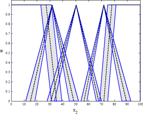

  

  IT2 membership functions for CPU load

• We order these and label them accordingly, e.g., with VL to VH labels representing Very Low to Low, Medium, High and Very High CPU loads.

Let a and b be the mean values of the interval end-points C P U _min and C P U _max of the labelled ranges with standard deviations σ _a and σ _b , respectively (see Fig. 6). For instance, for the Low, Medium and High label, the corresponding triangular T1 MF is then constructed by connecting left l, middle m and right r as follows:

$${} l = (a - \sigma_{a}, 0), m = ((a+b)/2,1), r=(b + \sigma_{b},0) $$

((30))

Accordingly, for Very Low and Very High processor load ranges that border 0 or 100 % on the normalized scale, the associated trapezoidal MFs can be constructed by connecting points as follows:

$$ (a - \sigma_{a}, 0), (a,1)(n,1),(b + \sigma_{b},0) $$

((31))

The labels above refer to utilisation rates of resources, with a maximum value being 100. So, irrespective of the concrete system, the labels are assigned to normalised utilisation ranges.

As indicated by the standard deviations in Fig. 6, there are uncertainties associated with the ends and the locations of the MFs. As an example, a triangular T1 MF might be defined follows:

$$ \begin{array}{l} l^{\prime} = (a-0.3 \times \sigma_{s},0)\\ m = ((a + b)/2,1)\\ r^{\prime} = (b +0.4 \times \sigma_{b},0) \end{array} $$

((32))

These uncertainties cannot be captured by T1 fuzzy MFs. In IT2 MFs on the other hand, the footprint of uncertainty (FOU) can be captured by the upper and lower MFs (UMF and LMF) for each range, see Fig. 8. A blurring parameter 0≤α≤1 can determine the FOU (see Fig. 6).

Fig. 8

Locations of the main points of IT2 MFs

Here, we use α=0.5. Parameter α=0 reduces IT2 MFs to a T1 MFs, while parameter α=1 results in fuzzy sets with the widest possible FOUs.

The fuzzy prediction process

After constructing the IT2 fuzzy sets with the MFs and the set of rules for the infrastructure load patterns, the prediction can then start to determine service quality estimations. The fuzzy prediction technique proceeds in a number of steps as follows (which we will explain in more detail afterwards):

• 1. The inputs comprising the workload are first fuzzified.

• 2. Then, the fuzzified input activates an inference mechanism to produce output IT2 FSs.

• 3. Decisions made through the inference mechanism are represented in the form of fuzzy values, which cannot be directly used as prediction results. The outputs are then processed by a type-reducer, which combines the output sets and subsequently calculates the center-of-set.

• 4. The type-reduced FSs are T1 fuzzy sets that need to be defuzzified in the last step to determine the predicted quality value q.

• 5. This value q is then passed back to the user as the predicted quality.

In the first step, we must specify how the numeric inputs u _i ∈U _i for the CPU utilisation rates are converted to fuzzy sets (a process that called “fuzzification” [18]) so that they can be used by the FLS. Here, we use singletons:

$$ \mu_{{\tilde{R}}_{1}} =\left\{ \begin{array}{ll} 1 &x= u_{i}\\ 0 & otherwise \end{array}\right. $$

((33))

For the defuzzification step, we use the construct of a centroid [21]. The centroid of a IT2 FS $\tilde {R}$ is the union of the centroids of all its embedded T1 fuzzy sets R _e :

$$ C_{\tilde{R}} \equiv \bigcup_{\forall R_{e}} c(R_{e}) = \left[ c_{l}\left({\tilde{R}}\right),c_{r}\left({\tilde{R}}\right)\right] $$

((34))

For the type-reducing step we use the center-of-sets construct [36]. The center-of-set (cos) type reduction is calculated as follows:

$$ Y_{cos} = \bigcup_{f^{l} \in F^{l}, y^{l} \in C_{{\tilde{G}}^{l}}} \frac{\Sigma_{l=1}^{N} f^{l} \times y^{1}}{\Sigma_{l=1}^{N} f^{l}} = \left[y_{l}, y_{r}\right] $$

((35))

where f ^l∈F ^l is the firing degree of mapping rule l and $y^{l} \in C_{{\tilde {G}}^{l}}$ is the centroid of the IT2 FS ${\tilde {G}^{l}}$. The centroids $c_{l}({\tilde {R}})$, $c_{r}({\tilde {R}})$ and y _l ,y _r are calculated using the KM algorithm from [21].

Fuzzy reasoning for quality prediction

Our quality mappings that encode the SWPs are in a multi-input single-output format. Because the log records of different services may not be similar, many patterns may be conflicting, i.e., we might have rule mappings with the same antecedent, but different consequent values. In this step, mappings with the same if-part are combined into a single rule. For each mapping in the patterns retrieved from the logs, we get the following for a sample rule R ¹:

$$ \begin{array}{l} IF ~ \left(x_{1} ~ is ~ {F^{l}_{1}}\right) ~ and ~ \ldots ~ and ~ \left(x_{p} ~ is ~ {F^{l}_{p}}\right), \\ THEN ~ \left(y ~ is ~ y^{({t_{u}^{l}})}\right) \end{array} $$

((36))

where ${t_{u}^{l}}$ is the index for the result. In order to combine these conflicting mappings, we used the average of all the responses for each mapping and use this as the centroid of the mapping consequent. Note, that the mapping consequents are IT2 FSs. However, when the type reduction is used, these IT2 FSs are replaced by their centroids. This means that we represent them as intervals $\left [ \underline {y}^{n}, \overline {y}^{n}\right ]$ or crisp values when $\underline {y}^{n} = \overline {y}^{n}$. This leads to rules with the following form for an arbitrary rule R ^l:

• IF the CPU workload (x ₁) is $\tilde {F}_{i_{1}}$,

• AND the network load (x ₂) is $\tilde {G}_{i_{2}}$,

• AND the storage utilisation (x ₃) is $\tilde {H}_{i_{3}}$,

• THEN q _i is the predicted value.

where C is the value of associated consequent, i.e., here a quality value for performance in ms, and ${w_{u}^{l}}$ is the weight associated with the u-th consequent of the lth mapping. Therefore, each q _i can be computed.

In a concrete example, we now illustrate the details of the prediction process. Assume that the normalized values regarding the three input parameters are x ₁=40, x ₂=50 and x ₃=55, respectively – see the solid lines for the workload in Fig. 9 as a sample factor. For x ₁=40, two IT2 FSs for the processor workload ranges F ₂=L o w and F ₂=M e d i u m with the degrees [ 0.3797,0.5954] and [ 0.3844,0.5434] are fired¹. Similarly, for x ₂=50, three IT2 FSs for the performance ranges G ₃=M e d i u m, G ₄=S l o w, and G ₅=V e r y S l o w with the firing degrees [ 0,0.1749], [ 0.9377,0.9568] and [ 0,0.2212] are fired. For x ₃=55 similar values would emerge. Intuitively, the lower and upper values of the intervals can be computed by finding the y-intercept of the solid lines in the figure, respectively, with the LMF and the UMF of the crossed FSs. As a result, six pattern mappings might result that are fired (here a sample is given):

$$ \begin{array}{l} M_{8}: (F_{2},G_{3},H_{1}), M_{9}:(F_{2},G_{4},H_{4}), \\ M_{10}:(F_{2},G_{5},H_{4}), M_{13}:(F_{3},G_{3},H_{2}),\\ M_{14}:(F_{3},G_{4},H_{1}), M_{15}:(F_{3},G_{5}, H_{2}) \end{array} $$

((37))

Fig. 9

IT2 MFs of for CPU workload ranges

The firing intervals are computed using the meet operation [17]. For instance, the firing interval associated to the pattern M ₉ for the CPU attribute is:

$$ m_{9} = \underline{\mu}_{\tilde{M}_{2}^{9}}(x^{\prime}_{1}) \otimes \underline{\mu}_{\tilde{G}_{4}^{9}}(x^{\prime}_{2}) = 0.3797 \times 0.9377 = 0.3560 $$

((38))

The output can be obtained using the center-of-set:

$$ \begin{array}{l} Y_{l}(40,50,55) = \\ \left[y_{l}(40,50,55), y_{r}(40,50,55)\right] = \\ {[}0.9296,1.1809{]} \end{array} $$

((39))

The defuzzified output can be calculated as follows:

$$ Y(40,50,55) = \frac{0.9296 + 1.1809}{2} = 1.0553 $$

((40))

Thus, we can finally calculate the predicted quality Y(x ₁,x ₂,x ₃) for all the possible normalized values of the input infrastructure parameters (i.e., x ₁∈[ 0,100], x ₂∈[ 0,100], x ₃∈[ 0,100] for CPU, storage and network).

Evaluation

Our proposed solution builds on a core pattern-based quality prediction solution that can be used for cloud configuration in an environment where there is uncertainty about concerns such as correctness or completeness. We have implemented an experimental test environment to evaluate the accuracy, efficiency and robustness of the solution in the context of uncertainty and dynamic processing needs.

Implementation architecture and evaluation settings

The implementation of the prediction and configuration technique covers different parts – off-line and on-line components:

• The pattern determination and the construction of the patterns-quality matrix is done off-line based on monitoring logs. The matrix is needed for dynamic configuration and can be updated as required in the cloud system. For the prediction, the accuracy is central. As the construction is off-line, performance overhead for the cloud environment is, as we will demonstrate, negligible.

• The actual prediction through accessing the matrix is done in a dynamic cloud setting as part of a scaling engine that combines prediction and configuration. Here the acceptable performance overhead for the prediction needs to be demonstrated.

• Uncertainties and noise are additional problems that arise in heterogeneous, cross-organisational cloud architectures. Robustness in the presence of these challenges needs to be demonstrated.

For both the accuracy and performance concern, we use a standard prediction solution, collaborative filtering (CF) as the benchmark, which is widely used and analysed in terms of these properties, cf. [11, 12] or [5, 6]. We have implemented a simulation environment with a workload generator to evaluate accuracy of the prediction approach and the performance of the prediction-based configuration. Test data is derived from sources such as [22] where quality metrics (response time, throughput) are collected for 5825 Web services with 339 users. We selected 100 application services from three different categories, each category either sensitive to data size, network throughput or CPU utilization. Figure 10 describes the testbed with the monitoring and SWP extraction solution for Web services. The primary concern is the accuracy of the pattern extraction and pattern-based prediction of performance for deployed services. Furthermore, as dynamic reconfiguration, i.e., auto-scaling, is an aim, also performance needs to be looked at.

Fig. 10

Evaluation architecture

We have tested our scalability management in Microsoft Azure. We have implemented a range of standard applications, including an online shopping application, a services management solution and a video processing feature to determine the quality metrics for different service and infrastructure configuration types. For the first two, we used the Azure Diagnostics CSF to collect monitoring data (Fig. 10). We also created an additional simulation environment to gather a reliable dataset without interference from uncontrollable cloud factors such as the network. Concrete applications systems we investigated are the following: a single-cloud storage solutions for online shopping applications [16] and a multi-cloud HADR solution (high-availability disaster recovery system [23]. This work has resulted in a record of configuration/workload data combined with performance data – as for instance shown in [16] where Figs. 3, 4, 5 and 6 capture response time for different service types and Figs. 7 and 8 show infrastructure concerns such as CPU and storage aspects. In that particular case, 4,100 test runs were conducted, using a 3-service application with between 25 and 200 clients requesting services. Azure CSF telemetry was used to obtain monitoring data. This data was then looked at to identify our workload patterns (CPU, Storage, Network) → Performance.

Cloud application workload patterns

A number of different application workload patterns are described in the literature [8, 13]. These include static, periodic, one-in-a-lifetime, unpredictable, continuously changing as in [8], or slowly varying, quickly varying, dual phase, steep tri-phase, large variation and big spike [13]. We need to make sure that this experimental evaluation does indeed cover the application workload pattern in order to guarantee general applicability. We followed [13] and induced these six patterns in our experiments. Based on the successful pattern coverage, we can conclude that the technique is applicable for a range of the most common situations.

We have implemented our prediction mechanism in different platforms. Work we described in [13] deals with how to implement this in an auto-scaling solution such as Amazon AWS where Amazon-monitored workload and performance auto-scaling metrics are considered together with a prediction of anticipated behaviour to configure the compute capabilities.

Accuracy

Reliable performance guarantees based on configuration parameters is the key aim – real performance needs to match the expected or promised one for the provider to fulfill the SLA obligations. Accuracy in virtualisation environments is specifically challenging [24] due to resource contentions because of the layered architecture, shared resources and distribution.

Accuracy of prediction is measured in terms of deviation from the real behaviour. The metric we use here is based on the mean absolute error (MAE) between prediction (SLA imposed) and real response time, which is the normal choice to measure prediction accuracy. Different characteristics of QoS have different ranges. Consequently, we use NMAE (the Normalized Mean Absolute Error) instead of the MAE. The smaller the NMAE, the more accurate is the prediction. We compare our solution with similar methods based on traditional prediction methods in terms of matrix density. This covers different situations from situations where little is known about the services (density is low) and situations where there is a reliable base of historic data for pattern extraction and prediction (high density).

In earlier work, we included average-based predications and classical collaborative filtering (CF) in a comparison with our own hybrid method (MCF) of matrix-based matching and collaborative filtering [7]. The NMAE of k=15 and k=18 (higher or lower k _s are not interesting as lower values are statistically not significant and higher ones only show a stabilisation of the trend) shows an accuracy improvement for our solution compared to standard prediction techniques, even without utility function and exponential smoothing, see Fig. 11. For this evaluation here, we also include time series (TS) into the comparison. For the evaluation, we considered some noisy data which cannot be in any pattern. We also removed invocation data and then predicted it using the CF, MCF and also the TS time series method from [25].

Fig. 11

Accuracy evaluation

We can observe that an increase of the dataset size improves the accuracy significantly. In all cases, our MCF approach outperforms the other ones by resulting in less prediction errors.

Efficiency overhead (runtime)

For automated service management in the context of cloud auto-configuration and auto-scaling we need sufficient performance of the extraction and matching approach itself. To be tested in this context are the performance of three components:

• 1. SWP Extraction from Logs (Matrix Determination)

• 2. Configuration-Pattern Matching (Existing Patterns)

• 3. Collaborative Filtering (Non-Existing Patterns)

For cases 1 and 2, we determined 150 workload patterns from 2400 usage recordings. We tested the algorithm on a range of different datasets extracted from a number of documented benchmarks and test cases. Com-pared to other work based on the TS and CF solutions, the matrix for collaborative computation is reduced from 2400 ^∗100 to 150 ^∗100, which reduces execution time significantly by the factor 16. For case 3, only when a matched pattern provides no information for a target service, the calculation for collaboration prediction is required, see Fig. 12, where we compare prediction performance with (MCF) as described in Sections ‘Workload patterns’ and ‘Quality pattern-driven configuration determination’ (using Algorithms 1 and 2) and without (CF) the pattern-based matrix utilisation.

Fig. 12

Performance evaluation

Robustness against noise and uncertainty

Exponential smoothing causes noise and results in some unavoidable errors. We need to demonstrate that our prediction solution is resilient against input noises, one of which is the estimation error through smoothing.

We experimentally evaluated the robustness against noise. We observed that the worst estimation error happens for large variation and quickly varying patterns and is less than 10 % of the actual workload. Based on this, we injected a white noise to the input measurement data (i.e., x ₁) with an amplitude of 10 %. We ran RMSE (root-mean-square error – measure of the differences between values predicted by a model or an estimator and the values actually observed) measurements for each levels of blurring, and for each measurement, we used 10,000 data items as input. We used different blurring values. Two observations emerged:

• Firstly, the error of control output produced by the prediction technique is less than 0.1 for the blurring levels.

• Secondly, the error of control output is decreasing when we configured the technique with a higher blurring.

A higher blurring as part of the smoothing leads to a bigger FOU in the uncertainty management, where FOU is a representative for the supporting levels of uncertainty. Therefore, the designer should make a choice in terms of the level of uncertainty that is acceptable. Note that in some circumstances an overly wide FOU results in a performance degradation. However, we can state that these observations provide enough evidence that robustness against input noise is maintained. Using IT2 FLS in the uncertainty management actually alleviates here the impact of noise.

Threats to validity

Some threats to the validity of the observations here exist. The usefulness of the approach relies on the quality of the workload patterns. While the existence of the patterns can be guaranteed by simply defining the individual ranges in the broadest possible way, thus resulting in some over-arching default patterns, their usefulness will only emerge if they denote sufficiently narrow ranges to allow the resources to be utilised in an equally narrow band. For instance, a band of 60–80 % is aimed at for processor loads.

While this has emerged to be possible for traditional software services that are computationally intensive or are typical text and static content-driven applications, multi-media type applications for instance with different network consumption patterns require more investigation.

Summary of evaluation

Thus, to conclude the evaluation, the computational effort for the dynamic prediction is decreased to a large extent due to the already partially filled matrix. As already explained, the performance of the pattern extraction and matrix construction (DBSCAN based clustering and collaborative filtering) can be computationally expensive, but can be done offline and only the matrix-based access (as demonstrated in the performance figure above) impacts on the runtime overhead for the configuration. However, as the results show, our methods overhead increases only slowly even if the data size increases substantially. Consequently, the solution in this setting is no more intrusive than a reactive rule-based scalability solution such as Amazon AWS Auto Scaling that would also follow our proposed architecture.

We specifically looked at the accuracy and robustness of the solution. The accuracy of the core solution based on the matrix is better than a traditional collaborative filtering approach. However, in cloud environments, other concerns needed to be addressed in addition. In order to address uncertainty due to different and possible incomplete and unreliable log data, we added smoothing and fuzzification. We have demonstrated that these features improve the robustness against external influence factors.

Related work

QoS-based service selection in general has been widely covered. There are three main categories of prediction-based approaches for selection.

• The first one covers statistical and other mathematical methods, which are often adopted for simplicity [1–3, 26, 27]. Others, e.g., in the context of performance modeling use mathematical models such as queues.

• The second category selects services based on user feedback and reputation [28, 29]. It can avoid malicious feedback, but does not consider the impact of SLA requirements and the environment and cannot customise prediction for users.

• The third category is based on collaborative filtering [11, 12, 30], which is a widely adopted recommendation method [31–33], e.g., [32] summarizes the application of collaborative filtering in different types of media recommendation. Here, we combine collaborative filtering with service workload patterns, user requirements and SLA obligations and preferences. This considers different user preferences and makes prediction personalized, while maintaining good performance results.

To demonstrate that our solution is an advancement compared to existing work on prediction accuracy, we had singled out two approaches for categories 1 and 3 for the evaluation above.

General prediction approaches

Some works integrate user preferences and user characteristics into QoS prediction [5, 11, 12, 30], e.g. [11, 12] propose prediction algorithms based on collaborative filtering. They calculate the similarity between users by their usage data and predict QoS based on user similarity. This method avoids the influence of the environment factor on prediction. However, even the same user will have different QoS experiences over time depending on the configuration of the execution environment or will work with different input data. Current work generally does not consider user requirements. Another current limitation of current solutions is low efficiency as we demonstrated. Our work in [13] is a direction based on fuzzy logic to take user scalability preferences into account for a cloud setting.

In [7, 34], pattern approaches are proposed. Srinivas [34] suggests pattern-based management for cloud configuration management, but without a detailed solution. Zhang et al. [7] is about bottom-up QoS prediction for standard service-based architectures, while in this paper QoS requirements are used to predict suitable workload-oriented configurations taking specifically cloud concerns into consideration. We added additionally exponential smoothing and utility functions and the cost analysis here, but draw on some evaluation results from [7] in comparison to standard statistical methods.

Cloud quality prediction and scalability

Various model-based predictive approaches are in use for cloud quality and resource management, including machine learning techniques for clustering, fuzzy clustering, Kalman filters, or low band filters, used for model updates which are then used for optimization and integrate with controllers Supporting cloud service management can automatically scale the infrastructure to meet the user/SLA-specified performance requirements, even when multiple user applications are running concurrently. Jamshidi et al. [13] deal with multi-user requirements as part of an uncertainty management approach, which is based on prediction as only exponent smoothing. Ghandi et al. [35] also leverage application level metrics and resource usage metrics to accurately scale infrastructure. They use Kalman filtering to automatically learn changing system parameters and to proactively scale the infrastructure, but have less of a performance gain than through patterns in our solution. Another work in this direction is [36], where the solution aims to automatically adapt to unpredicted conditions by dynamically updating a Kriging behaviour model. These deal with uncertainty concerns that we have excluded. However, an integration of both directions would be beneficial in the cloud. These approaches can add the uncertainty management solutions required.

Uncertainty management in clouds

Uncertainty is a common problem, particularly in open multi-layered and distributed environments such as the cloud applications. In [13], fuzzy logic is used to deal with auto-scaling in cloud infrastructures. We have adopted some of the principles here, but applied them to quality prediction here rather than resource allocation there. A similar fuzzy controller for resource management has been suggested in [37] based on adaptive output amplification and flexible rule selection. However, this solution is based on T1 FLS and does not address uncertainty.

The proposed method in this paper takes full account of user requirements (reflected in SLA obligations for the provider), the network and computational factors. It abstracts the service workload pattern to keep the service QoS steady. When user/SLA requirements are known, prediction-base configuration can be done based on matched patterns. This approach is efficient and reduces the computational overhead.

Conclusions

Web or cloud services [38] usually differ with respect to QoS characteristics. Relevant service-level qualities are response time, execution cost, reliability, or availability. There are many factors that impact on QoS [39]. They depend not only on the service itself, but also how it is deployed. Some factors are static, some are run-time static, the others are dynamic. Run-time static and dynamic factors like client load, server load, network channel bandwidth or network channel delay are generally uncertain, but can be influenced by suitable configuration in virtualised environments such as the cloud. Most factors can be monitored, and their impact on service-level quality can be calculated as part of a service management solution. Service management in cloud environments requires SLAs for individual users to be managed continuously through dynamic platform and infrastructure configuration, based on monitored QoS data.

We provided a solution that links defined SLA obligations for the provider in terms of service performance with lower-level metrics from the infrastructure that facilitates the provisioning of the service. Our solution enables cloud workload patterns to be associated to performance requirements in order to allow the requirements to be met through appropriate configuration. Note, that the investigation was based on the three quality concerns, but could potentially be extended to take other factors into account.

Performance management is still a problem in the cloud [4, 40]. While availability is generally managed and, correspondingly, SLA guarantees are made, reliably guaranteeing performance is not yet solved. Through a mining approach we can extract resource workload patterns from past behaviour that match the performance requirement and allow a reliable prediction of a respective configuration for the future.

What our approach signifies is the increased level of noise and uncertainty in cloud environments. Uncertainty emerges as different user roles are involved in configuring and running cloud applications, both on the consumer and provider side, and furthermore, data extracted from the cloud is uncertainty regarding its completeness and reliability as it might originate from different tools at different layers, possibly controlled by different providers or users. Noise occurs naturally in this setting, but is worsened by a need to apply for instance smoothing to address variability and detect trends.

There are wider implications that would still need more work for any solution to be practically viable. We started with three resource concerns, choosing one for each category. For the fuzzification, we focused on one concern to reduce complexity. Our experiments with concrete cloud platforms (Openstack and Azure) also show the need considerable integration work with platform services for monitoring and resource management.

In order to further fine-tune the approach in the future, we could take more infrastructure metrics into account. More specific cloud infrastructure solutions and more different use cases shall be used on the experimental side to investigate whether different patterns emerge either for different resource provisioning environments or for different application domains and consumer customisations [41].

Endnote

¹ The term ‘fired’ is commonly used for rules, generally assuming the consequents of the rules being actions that are fired. We have kept the term, but it applies here only to mappings to quality values.

References

Cardoso J, Miller J, Sheth A, Arnold J (2004) Quality of service for workflows and web service processes. J Web Semant 1: 281–308.
Kritikos K, Plexousakis D (2009) Requirements for Qos-based web service description and discovery. IEEE Trans Serv Comput 2(4): 320–337.
Ye Z, Bouguettaya A, Zhou X (2012) Qos-aware cloud service composition based on economic models In: Proceedings of the 10th International Conference on Service-Oriented Computing. ICSOC’12, 111–126.. Springer, Berlin, Heidelberg.
Chaudhuri S (2012) What next?: a half-dozen data management research goals for big data and the cloud In: Proceedings of the 31st Symposium on Principles of Database Systems. PODS ’12, 1–4.. ACM, New York, NY, USA.
Zhang L, Zhang B, Liu Y, Gao Y, Zhu ZL (2010) A web service Qos prediction approach based on collaborative filtering In: Services Computing Conference (APSCC), 2010 IEEE Asia-Pacific, 725–731.. IEEE, Piscataway, NJ, USA.
Zhang L, Zhang B, Na J, Huang L, Zhang M (2010) An approach for web service Qos prediction based on service using information In: Service Sciences (ICSS), 2010 International Conference On, 324–328.. IEEE, Piscataway, NJ, USA.
Zhang L, Zhang B, Pahl C, Xu L, Zhu Z (2013) Personalized quality prediction for dynamic service management based on invocation patterns. 11th International Conference on Service Oriented Computing ICSOC 2013. Springer-Verlag, Berlin, Germany.
Fehling C, Leymann F, Retter R, Schupeck W, Arbitter P (2014) Cloud Computing Patterns - Fundamentals to Design, Build, and Manage Cloud Applications. Springer, Vienna, Austria.
Zhang L, Zhang Y, Jamshidi P, Xu L, Pahl C (2014) Workload patterns for quality-driven dynamic cloud service configuration and auto-scaling In: Utility and Cloud Computing (UCC), 2014 IEEE/ACM 7th International Conference On, 156–165.. IEEE, Piscataway, NJ, USA.
Ester M, Kriegel HP, Sander J, Xu X (1996) A density-based algorithm for discovering clusters in large spatial databases with noise In: Proc. of 2nd International Conference on Knowledge Discovery and Data Mining, 226–231.. AAAI, Palo Alto, California, USA.
Shao L, Zhang J, Wei Y, Zhao J, Xie B, Mei H (2007) Personalized Qos prediction forweb services via collaborative filtering In: Web Services, 2007. ICWS 2007. IEEE International Conference On, 439–446.. IEEE, Piscataway, NJ, USA.
Zheng Z, Ma H, Lyu MR, King I (2011) Qos-aware web service recommendation by collaborative filtering. IEEE Trans Serv Comput 4(2): 140–152.
Jamshidi P, Ahmad A, Pahl C (2014) Autonomic resource provisioning for cloud-based software In: Proceedings of the 9th International Symposium on Software Engineering for Adaptive and Self-Managing Systems. SEAMS 2014, 95–104.. ACM, New York, NY, USA.
Kalekar PS (2004) Time series forecasting using holt-winters exponential smoothing. Technical report, Kanwal Rekhi School of Information Technology. IIT Bombay, Bombay, India.
Zhao H, Li X (2013) Resource Management in Utility and Cloud Computing. Springer, New York, USA. Springer Briefs in Computer Science.
Xiong H, Fowley F, Pahl C, Moran N (2014) Scalable architectures for platform-as-a-service clouds: Performance and cost analysis. 8th European Conference on Software Architecture, ECSA 2014. Springer-Verlag, Berlin, Germany.
Mendel JM (2007) Type-2 fuzzy sets and systems: An overview [corrected reprint]. IEEE Comput Intell Mag 2(2): 20–29.
Mendel JM, John RI, Liu F (2006) Interval type-2 fuzzy logic systems made simple. IEEE Trans Fuzzy Syst 14(6): 808–821.
Wu D (2012) On the fundamental differences between interval type-2 and type-1 fuzzy logic controllers. IEEE Trans Fuzzy Syst 20(5): 832–848.
Liang Q, Karnik NN, Mendel JM (2000) Connection admission control in atm networks using survey-based type-2 fuzzy logic systems. IEEE Trans Syst Man Cybern Part C Appl Rev 30(3): 329–339.
Karnik NN, Mendel JM (2001) Centroid of a type-2 fuzzy set. Inf Sci 132(1–4): 195–220.
Zheng Z, Zhang Y, Lyu MR (2010) Distributed Qos evaluation for real-world web services In: Web Services (ICWS), 2010 IEEE International Conference On, 83–90.. IEEE, Piscataway, NJ, USA.
Xiong H, Fowley F, Pahl C (2015) An architecture pattern for multi-cloud high availability and disaster recovery In: Workshop on Federated Cloud Networking FedCloudNet’2015.. Springer-Verlag, Berlin, Germany.
Gmach D, Rolia J, Cherkasova L, Kemper A (2007) Workload analysis and demand prediction of enterprise data center applications In: Proceedings of the 10th International Symposium on Workload Characterization. IISWC ’07, 171–180.. IEEE Computer Society, Washington, DC, USA.
Cavallo B, Di P, Canfora G (2010) An empirical comparison of methods to support Qos-aware service selection In: The 2nd International Workshop on Principles of Engineering Service-Oriented Systems.. ACM, New York, NY, USA.
Alrifai M, Skoutas D, Risse T (2010) Selecting skyline services for Qos-based web service composition In: Proceedings of the 19th International Conference on World Wide Web. WWW ’10, 11–20.. ACM, New York, NY, USA.
Zeng L, Benatallah B, HH Ngu A, Dumas M, Kalagnanam J, Chang H (2004) Qos-aware middleware for web services composition. IEEE Trans Softw Eng 30(5): 311–327.
Vu LH, Hauswirth M, Aberer K (2005) Qos-based service selection and ranking with trust and reputation management In: Proceedings of the 2005 Confederated International Conference on On the Move to Meaningful Internet Systems. OTM’05, 466–483.. Springer, Berlin, Heidelberg.
Li Y, Zhou MH, Li RC, Cao DG, Mei H (2008) Service selection approach considering the trustworthiness of Qos data. J Softw 19(10): 2620–2627.
Wu G, Wei J, Qiao X, Li L (2007) A bayesian network based Qos assessment model for web services In: Services Computing, 2007. SCC 2007. IEEE International Conference On, 498–505.. IEEE, Piscataway, NJ, USA.
Sarwar B, Karypis G, Konstan J, Riedl J (2001) Item-based collaborative filtering recommendation algorithms In: Proceedings of the 10th International Conference on World Wide Web. WWW ’01, 285–295.. ACM, New York, NY, USA.
Zeng C, Xing C-x, Zhou L-z (2002) A survey of personalization technology. J Softw 13(10): 1952–1961.
Xu HL, Wu X (2009) Comparison study of internet recommendation system. J Softw 20(2): 350–362.
Srinivas D (2013) A patterns/workload-based approach to the cloud. DIMS Lightning Talk, IBM. Online: http://www.slideshare.net/davanum/dims-lightningtalk.
Gandhi A, Harchol-Balter M, Raghunathan R, Kozuch MA (2012) Autoscale: dynamic, robust capacity management for multi-tier data centers. Trans Comput Syst 30(4): 14–11426.
Gambi A, Toffetti Carughi G, Pautasso C, Pezze M (2013) Kriging controllers for cloud applications. IEEE Internet Comput 17(4): 40–47.
Rao J, Wei Y, Gong J, Xu CZ (2011) Dynaqos: Model-free self-tuning fuzzy control of virtualized resources for Qos provisioning In: Quality of Service (IWQoS), 2011 IEEE 19th International Workshop On, 1–9.. IEEE, Piscataway, NJ, USA.
Pahl C, Xiong H (2013) Migration to paas clouds c migration process and architectural concerns. 7th International Symposium on Maintenance and Evolution of Service-Oriented and Cloud-Based Systems (MESOCA 2013). IEEE, Piscataway, NJ, USA.
Lelli F, Maron G, Orlando S (2007) Client side estimation of a remote service execution In: Proceedings of the 2007 15th International Symposium on Modeling, Analysis, and Simulation of Computer and Telecommunication Systems. MASCOTS ’07, 295–302.. IEEE Computer Society, Washington, DC, USA.
Jamshidi P, Ahmad A, Pahl C (2013) Cloud migration research: a systematic review. IEEE Trans Cloud Comput 1(2): 142–157.
Wang M, Bandara KY, Pahl C (2010) Process as a service distributed multi-tenant policy-based process runtime governance In: Proceedings of the 2010 IEEE International Conference on Services Computing. SCC ’10, 578–585.. IEEE Computer Society, Washington, DC, USA.
Acknowledgements
This research has been supported by the Fundamental Research Funds for the Central Universities of China (grant N130317005), by the National Natural Science Foundation of China (grant 61402090), and the Irish Centre for Cloud Computing and Commerce IC4, an Irish national Technology Centre funded by Enterprise Ireland, the Irish Industrial Development Authority, and by Science Foundation Ireland (International Strategic Cooperation Award Grant Number SFI/13/ISCA/2845).
Author information
Authors and Affiliations
Corresponding author
Additional information
Competing interests
The authors declare that they have no competing interests.
Authors’ contributions
LX and YZ have worked on the collaborative filtering solution presented in Sections Workload patterns and Quality pattern-driven configuration determination. LX (supervised by CP) has mapped this to the cloud computing context (Sections Quality-driven configuration and scaling and Pattern-driven resource configuration). PJ is the central contributor of Section Managing uncertainty (work that has been supervised by CP). CP is responsible for Introduction and Conclusions. All authors have contributed to the evaluation. All authors read and approved the final manuscript.
Rights and permissions
Open Access This article is distributed under the terms of the Creative Commons Attribution 4.0 International License (http://creativecommons.org/licenses/by/4.0/), which permits unrestricted use, distribution, and reproduction in any medium, provided you give appropriate credit to the original author(s) and the source, provide a link to the Creative Commons license, and indicate if changes were made.
About this article
Cite this article
Zhang, L., Zhang, Y., Jamshidi, P. et al. Service workload patterns for Qos-driven cloud resource management. J Cloud Comp 4, 23 (2015). https://doi.org/10.1186/s13677-015-0048-2
Received:
Accepted:
Published:
DOI: https://doi.org/10.1186/s13677-015-0048-2