Characterization and modeling of an edge computing mixed reality workload

Abstract

The edge computing paradigm comes with a promise of lower application latency compared to the cloud. Moreover, offloading user device computations to the edge enables running demanding applications on resource-constrained mobile end devices. However, there is a lack of workload models specific to edge offloading using applications as their basis.In this work, we build upon the reconfigurable open-source mixed reality (MR) framework MR-Leo as a vehicle to study resource utilisation and quality of service for a time-critical mobile application that would have to rely on the edge to be widely deployed. We perform experiments to aid estimating the resource footprint and the generated load by MR-Leo, and propose an application model and a statistical workload model for it. The idea is that such empirically-driven models can be the basis of evaluations of edge algorithms within simulation or analytical studies.A comparison with a workload model used in a recent work shows that the computational demand of MR-Leo exhibits very different characteristics from those assumed for MR applications earlier.

Introduction

Edge computing is a recent paradigm attracting interest from both researchers and industry practitioners [1]. It is driven by the variety of smart devices upcoming in new use cases that have strict latency requirements not satisfied by the cloud computing paradigm. In an edge network, resources such as computation or storage are located in close vicinity to the end users, at the edge of the network.

The envisioned application areas for edge computing are very diverse: smart agriculture [2], smart city [2, 3], healthcare [3, 4], and connected vehicles [4–7], among others. However, most resource management studies do not consider specific application load characteristics. Either they do not use different application types in their evaluation, or even when they do, the load is not based on a real application, but on a standard theoretical abstraction of what the load may look like [8].

One application area that is especially relevant for edge computing due to its latency requirements and high computational demand is mobile mixed reality (MR). Several surveys have highlighted this application area [3–6] but few open-source applications are available for studies. Those freely available are not configurable in order to study variations of offloading strategies and with no released code base. We contribute to filling this gap by illustrating the benefit of an open-source framework for studying full or partial offloading of mixed reality to the edge.

Our work with mixed reality in an edge computing context aims at answering the following research questions: Is offloading all MR-related computations to the edge with current technology feasible? If not, where are bottlenecks, and where is the potential for improvement of quality of experience highest? Once we have understood the different elements in a real application workload, can this be successfully used to generalise a statistical workload model for future edge studies or for meaningful analysis of resource allocation algorithms?

In our earlier work [9], we started answering those research questions by proposing MR-Leo, a generic framework for offloading video streams to the edge, released as an open-source code base. In that paper a couple of alternative hardware platforms were used as comparative platforms, and a couple of communication protocols and video compression formats were used for transporting the frames. This paper is a substantial extension of the above paper with the following contributions:

• A vehicle for a general study of the edge resource demand of MR applications via the open source MR-Leo prototype

• A workload characterization and modeling approach used for understanding the workload created by MR-Leo as an exemplary MR application

• An application model and a statistical workload model based on MR-Leo that can be used for simulation studies, and demonstrating its usefulness compared to a theoretical model in the context of edge orchestration.

The new studies highlight the necessity to create edge application models that are based on real implementations before being used in simulation studies, so that meaningful and relevant results can be obtained.

In particular, this study clearly illustrates that the CPU resource demand of the prototype is strongly influenced by the performance of the point cloud algorithm, and that the task arrival pattern is important for MR workloads.

The paper is structured as follows. First we present related works and introduce the problem tackled in this paper: offloading mixed reality to the edge. Then, we briefly present the MR-Leo prototype and highlight some earlier results from the conference paper [9] in the section “Performance evaluation”. The reader already familiar with that paper can start reading from section “Focus on the edge resource demand”, where we investigate the resource demand of the prototype at the edge. Next, we present a characterization and modeling approach used for analyzing the workload created by the prototype. The results of the analysis are then presented, first the understanding obtained through characterization and then an MR application model and an MR workload model. In the following section, we discuss how these models differ from previous ones, their impact on earlier published results, and the benefits and relevance of the chosen approach. Finally, we conclude the paper and describe future works.

Related works

In this section, related research is presented, first with regards to offloading mixed reality to the edge, and then regarding edge workload characterization and modeling.

Offloading mixed reality to the edge

When focusing on the edge computing area, there is active research on MR and especially AR as it can be considered as one of the killer applications for the edge [10].

In a recent survey, Chatzopoulos et al. [11] describe different alternatives for offloading the heavy computations required by mobile augmented reality (AR). Offloading to the edge is one of the possibilities investigated by current works, together with offloading to a companion device in close proximity or to the cloud. The current research can also be separated into two different categories based on what exactly is offloaded: either both the computing and the rendering work, or only the computing, the rendering being performed locally. In this paper, both rendering and computing are offloaded to the edge.

Several other works also address the offloading of MR applications. While this study considers one edge device computing both the rendering and the encoding, Zhang et al. [12] study the separation of the encoding and rendering tasks onto different edge devices in order to improve quality of service compared to when encoding and rendering are performed in the same edge device. On the other hand, our work includes a real user device whereas Zhang et al. used simulated user demand to evaluate their optimized solution.

Another option is to perform some degree of pre-processing at the end device as in the work by Zhang et al. [13]. Their system called Jaguar can recognize an object using machine learning (ML) with low latency, after an offline training phase of the edge part and pre-processing of the video frames on the end device. In our platform for resource studies, no pre-processing is performed at the end device.

A further option is to consider that the device creating the video stream is different from the one displaying the MR-enhanced stream as in the NEAR framework proposed by Trinelli et al. [14]. They investigated Network Function Virtualization for computation acceleration for MR at the edge. Their specific MR application was object detection using machine learning techniques.

Closer to the work presented in this paper in terms of the offloading alternatives chosen, Chen et al. [10] study prototypes for seven different wearable cognitive assistance applications implemented using their Gabriel platform [15]. They study the latency of AR applications in different setups (offloading the application to the edge or to the cloud, using 4G or WiFi for the first hop connection), and using different hardware (mobile phones and smart glasses). However, our work uses a novel type of application (i.e. one that outputs to the user an enhanced video stream and not only visual or auditive indications), and presents an extensive study about the protocols and video compression formats used for the communication link, as well as the edge resource demand (in this paper). In contrast, Gabriel only uses MJPEG over TCP for the communication link and focus on latency only.

A similar study of offloading AR to the edge was presented recently by Bachhuber et al. [16]. They focus particularly on bringing down the end-to-end (E2E) delay on the end device by optimizing the encoding and decoding steps. They achieve a E2E delay of 83.5 ms, which is comparable to state-of-the-art AR application running locally on a smartphone such as Google ARCore or Apple ARKit. However, those low latencies are achieved by using a Gigabit Ethernet connection between the end and the edge device as well as a laptop as the end device. While future 5G stations are likely to have much better capacity than our experimental wireless setup, their capacity limits will perhaps be somewhere in between our communication channel and the one in that paper. The limitation of a mobile wireless end device will most likely persist though. Moreover, the application and the video stream used in the evaluation are not publicly released, preventing a fair comparison with MR-Leo.

Edge workload characterization and modeling

Most of the research works in edge resource management use simulation or analytical tools [8], which requires a model or a trace of the application considered. Although there is usually a need for a load profile for edge applications, the currently used models are not based on real applications but on characteristics that are derived from how such an application is expected to behave.

Works on benchmarking can be useful for describing application characteristics. In the edge computing area, those efforts are at an early stage. Current edge benchmarking efforts, e.g. that by McChesney et al. [17] and Toczé et al. [18], have application characteristics described in broad terms such as “bandwidth/computational intensive” or “close/far”. This is not detailed enough to be used in simulations or analyzes that provide deeper insights.

Some benchmarks focusing on cloud applications have started looking at workloads using edge like the microservice benchmark from Gan et al. [19]. Out of 6 open-source applications, they propose one drone swarm coordination service where part of the services are run on the drones. In their work, only results regarding tail latency are presented for the six applications. Tail latency is the latency of the lowest instances of the service. This is not enough to be used in other applications without running the actual code.

Among recent edge works using MR applications, Sonmez et al. [20] present three applications (including an MR application) to be run in their EdgeCloudSim simulator. These are mostly described in broad terms such as “high/small” for the CPU resources required and the amount of data transferred. Apart from the upload/download data size for the MR application that are derived based on a chosen image/text metadata size, the other numerical data is not explicitly justified. Mukherjee et al. [21] summarize different mathematical models used for capturing e.g. latency in edge computing in earlier works [22, 23]. Such models are useful but they also have limitations. Since they are generic they do not capture the specificity of different application types, e.g. they include assumptions such as task arrivals following a Poisson process which is questionable in the case of MR, and they do not provide numerical values based on empirical measurements.

Other works build their analytical models on data coming from application profiling, such as Zhang et al. [12], who study the resource demand of the colocated encoding for MR using three metrics (CPU utilization, GPU utilization and network transmission). However, this study presents only numerical data averaged over 90 seconds, which can hide variations of the resource demand over this period that are relevant to model.

Our work combines and enhances the above approaches, by a methodical generation of workload models, similar to earlier works in the cloud computing area. It aims to ground our MR synthetic model in profiled edge application data in order to create a realistic workload model.

Earlier attempts to do this in a cloud context are now briefly mentioned. Shen et al. [24] performed a statistical characterization of business-critical workloads for cloud computing. They used three different statistical instruments, namely basic statistics, correlations and time-pattern analysis. They found interesting findings about how such a workload behaves. Their objective was improving the resource usage effectiveness and handling peak loads in clouds. We share the same ambition, with application to mixed reality offloaded to the edge. This work differs from the one considered by Shen et al. on several points: 1) we study a specific time-critical application area, 2) our study is based on a reconfigurable open-source prototype and not a real deployment as those do not yet exist (or not freely available).

Talluri et al. [25] propose a characterization of real workload traces from Big Data applications in a cloud computing context. They perform statistical analysis of the data and study different aspects such as long-term trends, impact of file types, and clustering. The method used in this paper shares some of the statistical tools used by Talluri et al., as they have shown to give relevant insights about the workload characteristics.

MR at the edge

In this section, the concept of offloading is first presented. Then, an MR application as a means of understanding and building workload models is introduced. We present here an overview of the MR-Leo prototype developed earlier with enough details that make the current paper accessible when the application is used as a vehicle of generating workload models.

Offloading to the edge

One of the main ideas of edge computing is to use the resources present at the edge level to perform computation instead of using the resources present inside the end device. Using the edge CPU as a resource instead of the user (end) device, i.e. offloading, has several benefits. First, it makes it possible to run applications that the end device is not capable of due to limited resources. Even if execution at the end device would be possible from a performance or thermal perspective, doing it elsewhere should save battery, so that the end device can be used for a longer period. Executing at the edge may also enable to share the results between users in order to provide a faster service, or higher resilience in case a node becomes non-functional.

Hence, in an offloading scenario there will be a variety of requests for execution sent to the edge devices from the end devices. This is what we consider as the edge workload and study in this paper.

MR case study

Mixed reality is an umbrella term for describing the part of the reality-virtuality continuum [26] that combines reality and virtuality, designating any technology that manages mixes of reality and virtuality. It includes for example augmented reality. An example of an MR output where the Android mascot is added in a library environment is shown in Fig. 1.

Fig. 1

Example of mixed reality output

An MR application consists of different components and its workflow (illustrated in Fig. 2) can be summarized as follows:

• 1. Some sensor input (such as a video stream) is gathered.

  Fig. 2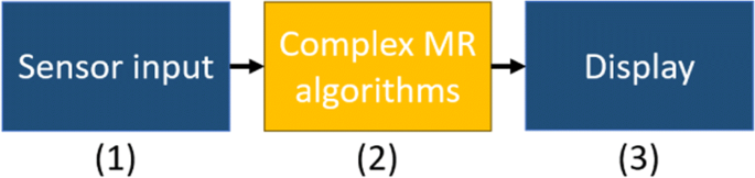

  

  MR application workflow

• 2. Complex MR algorithms are executed to create a model of the environment present in the input stream and add the virtual elements (VEs).

• 3. The resulting MR-enhanced scene is displayed back to the user.

In the scenario considered in this paper, the second step is offloaded to the edge while the other two are still performed on the end device.

MR-Leo prototype

We implemented our own interactive MR application using edge computing, called MR-Leo, short for Mixed-Reality Linköping edge offloading, which is released open-source^1,2. This implementation was a required step before being able to perform the characterization presented in this study. To the best of our knowledge, no MR application offloading all the MR computations (i.e. step 2 above) to the edge is currently available open-source.

MR-Leo uses open-source frameworks such as Gstreamer³ for transmitting video, ORB-SLAM2 [27] for creating the environment model using MR technologies, and Pangolin⁴ for rendering the MR graphics to an image feed. Among the insights gained during the development process, it can be highlighted that best quality of service is achieved when it is possible to process a video frame before the next one arrives to the edge and when frames arrive regularly. More details about the MR-Leo implementation and insights gained during the development phase can be found in [9].

Performance evaluation

In this section, the main insights from the performance evaluation presented in our conference paper [9] that this paper extends are presented. Readers interested in the further details of the evaluation setup or all the alternative configurations studied therein are referred to the mentioned paper.

Evaluation setup

The full experiment scenario consists in capturing a dynamic scene with a smartphone and sending the captured video stream to an edge device that will analyze it to create a point cloud. Then, the stream is augmented with the output of the deployed MR framework. In this case, it consists of a visualization of the point cloud, i.e. the constructed virtual representation of the scene, sent back to the smartphone. Figure 3 presents this scenario. We can see that in addition to the steps present in Fig. 2, the prototype requires additional steps related to the video transmission between the end and the edge devices.

Fig. 3

MR scenario used in the experiments

A variant of this scenario is when the smartphone user presses a button in order to add a virtual element to the scene. In this case, the steps performed are a bit different, as shown with green elements on Fig. 3. The main difference is that the uplink transmission now only consists of a message indicating the element to be added, and not of the full video stream.

In both scenario variants, the video is streamed one frame at a time at the rate at which the stream is captured (i.e. 30 frames per second). When a frame is received at the edge it goes through the MR algorithms and the resulting frame is transmitted back to the end device as soon as it is available.

The performance evaluation includes comparing different configurations that can be used for the scenario presented in Fig. 3.

Each experiment was conducted 30 times for the same configuration in order to mask any network interference or computing hardware performance fluctuations. In order to ensure reproducibility between the runs, a video play-back is used instead of the actual camera feed on the end device. The test video used is 60 seconds long and is set up in an indoor environment. The full video is available online⁵, and has a resolution of 640x480 pixels and a frame rate of 30 fps.

In the performance study, in order to detect when a specific frame comes back to the end device (to be able to measure round trip time or to detect that a virtual element has been added), we use artificially added rows of pixels with bright colors not present in the original video on 11 specific frames spread in the video (which had in total 1814 frames). This technique enables to easily detect those frames in a very lightweight manner (by only having to check the color of some specific pixels) that does not require to track every individual frame (which would be impractical) or use complex object recognition algorithms (which would significantly increase the measured times in a non-deterministic manner). This frame detection approach has a negligible probe effect which can be isolated.

The experiments were first run with the following edge device and end device, hereafter called the baseline devices.

The baseline edge device is a Lenovo Thinkpad T450s laptop. The laptop runs Ubuntu 18.04 and has 12 GB RAM and an Intel Core i5-5200U CPU (2.2 GHz, 2 cores, 4 threads), which is classified as a high mid-range CPU as of July 2019 [28]. For the end device, the baseline device is an LG G6 smartphone running Android 8.0 and equipped with the Qualcomm Snapdragon 821 mobile platform. It contains a Qualcomm Kryo CPU (2.4 GHz, 4 cores) and 4 GB RAM.

In addition, a second edge device was considered in some of the results highlighted in this paper: it is an HP Elitebook 840 G5. It runs Ubuntu 18.10 and has 16 GB RAM and an Intel Core i7-8550U CPU (1.8 GHz, 4 cores, 8 threads), which is classified as a high end CPU as of July 2019 [29], thus being more powerful than the baseline device.

The experiments were performed over a local network set up using an Asus RT-N12 router disconnected from the Internet. The edge device was connected to the network using an Ethernet cable and Gigabit Ethernet (1000 Mbit/sec), and the end device was connected using an 802.11n wireless network. The end and edge devices were placed within one meter from the network gateway, and the same positions were used for all tests using the same devices.

Performance metrics

Two different metrics were used when evaluating end-to-end (E2E) latency:

• 1. the time elapsed between the moment the end user presses the “Add virtual element” button and the moment when the virtual element appears on the display (Steps (a-bis) to (j) on Fig. 3) or time to virtual element (T2VE),

• 2. the time it takes for a captured video frame to be displayed with the MR enhancement on the display (Steps (a) to (j) on Fig. 3), or frame round trip time (FRTT).

As the FRTT requires the video frame to be transmitted both to the edge and back, more resources are used on the communication link than for T2VE. This communication part has been shown to account for 92% of the whole FRTT. At the same time, the latency requirements on frame handling are critical for the application to be perceived as real-time. It is therefore crucial for performance to bring the FRTT as low as possible. Therefore, this performance metric is the most relevant one for studying the overall performance of the MR application, when the MR framework is performing as expected. In this normal scenario the MR framework is able to create a point cloud from the scene. By design and as verified by measurements, the T2VE metric will always show lower latency than FRTT when there is no problem in the point cloud creation.

Therefore, only results relating to FRTT are presented in this paper. For reading about the results regarding T2VE or throughput, the readers are referred to [9].

Alternative configurations and highlights

In our previous work, different configurations were tested with regards to the protocol and video compression format used for the communication link, as well as different hardware for the edge and end device. We highlight some outcomes in this section.

The two configurable parts of the communication link for which different alternatives were evaluated were the protocol used for the transmission and the video compression format used for encoding/decoding of the video stream.

Figure 4a shows the cumulative distribution function (CDF) for the configuration where TCP is used as the transmission protocol and H.264 as the video compression format. Those are widely used and act as a performance baseline. At the 90th percentile, the FRTT is 538 ms, which is more than 5 times higher than the limit of 100 ms that is perceived as an “immediate answer” according to the literature [30]. Therefore, the first insight from the measurement study was the need for other alternatives for decreasing the time spent in the transmission part of the application (e.g. 5G transmission).

Fig. 4

Latency CDFs for FRTT in different configurations

An alternative to replace TCP is UDP. The FRTT results are shown in Fig. 4b. Using this protocol improved the FRTT at the 90th percentile by 27% (392 ms instead of 538). However, this comes at the cost of higher bandwidth required for the communication link and the MR framework has to tolerate potential loss of frames.

The higher bandwidth required for UDP is due to the fact that with TCP only the difference between frames needs to be sent most of the time, so the amount of data transmitted can be reduced without affecting the image quality used as input in the MR framework. However, UDP requires to transmit complete frames all the time because some could be lost, and the MR framework cannot track points on incomplete images. Therefore, to be able to track the same number of feature points by the MR framework, more data needs to be transmitted when using UDP. Through measurements, we found that a suitable and stable number of feature points (around 250) can be achieved for a bandwidth of 2000 kbit/sec for TCP and 4000 kbit/sec for UDP.

Using MJPEG instead of H.264 on the downlink was the next configuration to explore. The results for the FRTT are presented in Fig. 4c and show a 54% reduction at the 90th percentile (down to 245 ms). This is very promising, especially considering that only the compression format for the downlink was modified. Indeed, there were performance issues (introduction of a significant delay) when using the jpegenc Gstreamer plugin for MJPEG streaming in the uplink, due to the way the plugin is implemented. This prevented us from fully studying MJPEG in the experiment. If this technical limitation is lifted, the total transmission time is expected to go down even further.

In addition to the time spent in the communication link, another aspect of the application was identified as a contributor to increased latency: frames queuing in the communication service before being processed for point cloud and graphics. This can be seen in Fig. 5 that shows the part of the average FRTT dedicated to the MR-related processing at the edge, i.e. excluding transmission and encoding/decoding to make this queuing aspect visible.

Fig. 5

Latency breakdown of the MR-related edge processing for different configurations

Although it is possible to parallelize some parts of the MR calculations, e.g. separate threads to handle video reception, frame analysis for the point cloud creation, addition of graphics into frame, and video sending, and indeed this is how it is implemented in MR-Leo, the way the point cloud algorithms work in ORB-SLAM2 require that frames are analyzed sequentially in the order they were captured. This analysis takes place as a pipeline comprising several operations. Therefore, it is not yet possible to process several frames in parallel in the same operation within the pipeline to reduce the queuing time. Different frames are processed in different pipeline parts one at a time.

In order to reduce the queuing time, the experiment was therefore run on the second more powerful edge device (presented in the experiment setup section) and the results are labeled as High-end on Fig. 5. They show that using a more powerful edge hardware contributes to reducing the frame queuing time as well as the MR framework execution time. However, the graphic rendering part was not impacted, probably because graphics accelerators would be required for this and the current prototype configurations do not support this.

Focus on the edge resource demand

In addition to studying the response times of the prototype, it is also interesting to look at its resource demand. We focus on the edge part of resource demand as this is where the computationally intensive parts of the application are executed, as explained earlier.

Three resource types are considered: computation, communication and memory demand. The main focus is on the computation demand, which is the most common resource considered in the literature [8].

Data collection and analysis method

The data collection process for this study was separated into two steps. First, we observed the resource demand of MR-Leo on the edge device when running the experiments described in the “Performance evaluation” section. The aim was to gather data and insights while keeping the measurement complexity low. While it was possible to collect the required data for communication and memory demand in this first step, only limited insights about the computation demand were gathered. Therefore, a deeper study in performed in the second step with more detailed experiments in order to get a better picture of the computation demand.

For the first step, MR-Leo is instrumented to record the CPU and the memory use at every second on the edge device. This is done using the Linux top tool as it is a lightweight tool already part of the standard Ubuntu distribution. This tool enables gathering of the required memory demand data and the CPU utilization values through the experiments. This keeps the impact on application execution environment to a minimum.

However, while the top granularity level (per second) is satisfactory for the memory demand, it is too coarse for the computation demand, as a video frame is sent every 33 ms to the edge. Therefore, to get more fine-grained data for the computation demand, a second study step was performed. In this step, the aim is to collect the number of executed instructions per video frame. To obtain it, a separate instrumentation of the application code was performed using a custom code building on the Intel Pin tool⁶ for binary code analysis. This tool enables to count the number of instructions executed between two points in the source code. In this second study step, the tool is used to count the number of instructions executed when processing a frame in the class that feeds the decoded frames to the MR function. Since binary code analysis significantly slows down the execution of the application, a dedicated set of experiments was performed for this second step.

The experimental data presented in this section was obtained by running the experiments on the high-end edge device (HP) used for the performance evaluation. Two sets of experiments are used, one for each step presented above: first using the video play-back with automatic user input as in the previous section (later denoted as the reference video). Second, using a mocked smartphone client, i.e. the video frames are directly used as input on the edge server, due to the slow down created by the binary analysis tool. In this second experiment set, separate runs were conducted for video input alone, and for video and user input combined.

The experimental data gathered was analyzed using different statistical techniques. First, the data obtained is plotted using histograms in order to visualize how the data behaves. In addition, descriptive statistics such as the mean, median, maximum and minimum values are presented. The presence of one or several modes in the data is also studied. The mode of a set of values is the value appearing most often [31]. It appears as a local maximum in the probability density function of the data distribution. In some distributions, there are several such local maxima. In this case the data is multimodal and the different modes can be identified by statistical tools. When necessary, the Kolmogorov-Smirnov (KS) test and Pearson’s chi-squared test are used. These are two statistical tests for studying different similarity indicators that are suitable for comparing two distributions. The KS test measures the maximum difference between two cumulative distribution functions and its result can be seen as describing the divergence of the two distributions, and the Pearson’s chi-squared test, measures the difference between the histograms of two empirical distributions [25]. For this statistical analysis, we used a significance level of 5%.

Computation demand

Characterizing the computation demand is not a straightforward task. In the literature, the computation demand is sometimes not quantified but described in generic categories such as “High” or “Low” [17, 18]. When it is quantified, the metric chosen varies and the numbers are provided without explaining how they were obtained. In this study, two metrics are used for quantifying the computation demand: the number of cores used and the number of instructions executed for running a task.

Number of cores

For characterizing the CPU load of MR-Leo, the CPU use during running the edge processing part of the application was logged on the edge device. The result is that the application requires the power of three cores. This can be seen in Fig. 6, showing a histogram of the CPU usage values recorded during 30 experimental runs. On the figure, the maximum CPU utilization goes up to 226%, i.e. the application requires the equivalent of two cores utilized at 100% and a third one utilized at 26%, so the power of three cores is needed⁷.

Fig. 6

Measured CPU use per second

Since the top tool needs to be started/ended a bit before/after the video is streamed from the end device, the measurements include a few seconds where MR-Leo is almost idle. That is the reason for the leftmost bar on Fig. 6.

Number of instructions per video frame

With regards to the number of instructions executed and as described in the data collection method section, a dynamic binary analysis is performed with a custom adapted tool based on Pin.

The analysis was run 5 times on the reference video stream. Figure 7 shows a histogram of the number of instructions per frame over the 5 runs. Basic statistics over the 5 runs, are presented in the first row of Table 1. On the histogram, it can be seen that the numbers of instructions are not spread homogeneously over the span between the minimum and the maximum values. On the contrary, the data exhibits two modes: one at 158.43 million instructions (MI) and a second one at 310.03 MI.

Fig. 7

Measured number of instructions per frame for the reference video

Table 1 Basic statistics for the instruction count (MI)

When plotting the data for each run separately, the shape of the histogram is similar. In order to quantify this similarity, the output of each run is compared to the other ones using the Pearson’s chi-squared test. Twelve bins were considered for grouping the data. The tests indicate similarity between the distributions obtained from the different runs (with p-values between 0.23 and 0.24).

We conjecture that the two modes of the distribution, i.e. the two levels of computational intensity, correspond to two situations in which the application can be: 1) it needs to create a point cloud, and 2) it needs to update it. The first situation being more computationally intensive than the second one. In order to test this, two additional series of tests were conducted with two other videos⁸.

The first one shows different objects disposed on a table (referred to as the object video) while the second one is shot in an outside environment on the campus of Linköping University (referred to as the campus video). The two additional videos contain the same number of frames as the reference video. When using MR-Leo, those two videos exhibit different behaviours compared to each other and to the reference video. For the object video, a point cloud can be found by the MR-Leo application and once found, is kept until the end of the video. On the contrary, a point cloud can never be found for the campus video since the scene is too complex for the MR framework used (although it reflects the state-of-the-art, as mentioned earlier). The reference video exhibits a behaviour in between those two extremes, with a point cloud being created but lost for a while around 30 seconds, and then recovered. When the point cloud cannot be created, MR-Leo sends back the received frame without any modification and the user sees the original stream.

When plotting the histogram of 5 runs each using the three videos, it can be seen that the number of instructions executed is different in the three different scenarios captured by the three videos. Figure 8a shows the histogram for the campus video. This histogram is unimodal with a mode at 287.46 MI. Figure 8b shows the histogram for the object video. This histogram is actually trimodal, with two modes close to each other (160.45 MI and 172.24 MI) that are aggregated in the first bin of the histogram, and a third one at 269.59 MI, containing only 13% of the data values. Basics statistics for the campus and object videos can be found in Table 1 and compared to the statistics of the reference video (in row 1).

Fig. 8

Measured number of instructions per frame

The results here corroborate the conjecture made, i.e. that the right mode of the distribution corresponds to when MR-Leo needs to create a point cloud (illustrated with the campus video). On the contrary, the left mode corresponds to when MR-Leo only needs to update the point cloud (illustrated with the object video).

Number of instructions in presence of user input

The next aspect we study is the difference in terms of instructions executed depending on whether user input has been sent to the edge node or not. The experiment performed for obtaining the number of instructions per video frame is adapted to include an automatic trigger of a user input adding a virtual element during 100 frames, and then removing the virtual element during the next 100 frames and so on during the whole experiment length. This adapted experiment is run 5 times.

We plot the histogram of the frames including a virtual element on Fig. 9a and of the frames not including a virtual element on Fig. 9b. The hypothesis here is that the extra computation needed to render the virtual element (a simple 3D object) is low compared to the rest of the MR calculations executed for every frame. The two distributions are compared using the KS test and Pearson’s chi-squared test. The KS output is 0.028 and the p-value obtained is 0.086 for the Pearson’s chi-squared test. This indicates that the two distributions are not significantly different.

Fig. 9

Measured number of instructions per frame

Note that, due to the way that the MR framework used works, every run of the experiment is unique and the quality of the point cloud created (i.e. the distribution between the two modes) are similar but unique to each run. The point cloud quality depends on how well the MR framework succeeds into identifying and keeping track of feature points, as well as which feature points it chooses during a specific run. A lower point cloud quality (e.g. a bad choice of feature points) will lead to a need for more recalculations, hence a higher computational demand. This is why, for example, the two modes in this experiment have similar bar heights, compared to Fig. 7 where the left mode had a higher bar than the right one.

Communication demand

Here it needs to be highlighted that MR-Leo will have an almost symmetric amount of data transmitted for upload and download, contrary to what is sometimes assumed for MR applications (e.g. in [32]). This is because all the MR parts, including rendering, are offloaded to the edge. Thus, a full frame is transmitted to the edge, and also a full frame back to the end device. The only part that is not symmetric is the one corresponding to user tasks, as that are only transmitted from the end device to the edge device. Those tasks however represent only a tiny fraction of all tasks.

Regarding video tasks, we look at their characteristics when generated on the end device. The reference video stream is an example scenario for the MR-Leo application. This video stream includes 1814 frames for a size of 75.5MB, which corresponds to each frame having a size of around 41kB before encoding. How much data is going to be actually transmitted between the end device and the edge device will depend on the video compression standard chosen. Modelling the behaviour of different compression standards (such as H.264 or MJPEG that are included in MR-Leo) is relevant but out of the scope of this paper.

For user tasks, the size of a request is fixed and can be obtained by studying the MR-Leo implementation. It consists of 60 bytes: 10 bytes for the header and 50 data bytes. The user tasks are not encoded so their size is independent of the compression format used.

Memory demand

MR-Leo is implemented so that it does not store data permanently on the edge server but only requires memory during run time. Figure 10 shows a histogram of the memory usage measurements, with a measurement taken each second during 32 experimental runs. This includes the memory used by the application before the end device connects, during the time it is connected, and after the end device disconnection.

Fig. 10

Histogram of the memory usage of the MR application

Two levels of memory occupation clearly appear in Fig. 10. The first one, around 1 281 MB (on the x axis) corresponds to the memory usage of the application when no end device is connected. The second, at on average 3 735 MB (with a standard deviation of 82 MB) corresponds to the memory usage when an end device is connected, i.e. representing the size of the application and the environment model associated to the connected end device. During the connection time of the end device, the memory occupied usually increases and decreases by a few tens of MB, but without any obvious pattern related to the video stream used for the test.

Workload characterization and modeling

The previous two sections studied the performance and resource demand of different parts of MR-Leo. In this section, the approach used for characterizing and modeling the workload created by MR-Leo is described. The obtained insights and models derived from MR-Leo can then be used in studies that cannot use the implementation, e.g. in large scale simulations of many such applications running in parallel in edge computing simulations.

We focus on characterizing and modeling the workload incoming to the edge (i.e. the demand), so that the performance of potential edge algorithms or MR components can be evaluated. For example, how long the tasks generated by the workload will take to complete is dependent on the system under evaluation (and how it is simulated in different simulators). Note that we consider here the case where each end device will run an instance of the application in isolation (e.g. a MR-Leo container).

There are a lot of aspects that could be studied when performing workload characterization. Our objective is that the characterization and modeling presented in this paper is of relevance for researchers and developers of edge computing platforms and algorithms. The resulting models are intended to be used for evaluating algorithm or tools, e.g. resource allocation algorithms and orchestration tools.

Overview

Our proposed workflow is inspired by workflows used for characterizing other type of workloads such as big data applications [25]. In addition to describing the behaviour of the application, i.e. characterizing it, it also includes modeling it in order to be able to synthetically generate a workload that will exhibit the same characteristics in repeated experiments. An overview of the characterization and modeling workflow is presented in Fig. 11.

Fig. 11

Characterization and modeling workflow

As an input, the workflow takes an application and relevant load indicators to gain insights about (blue pentagons). The characterization part of the workflow is composed of three main steps represented by boxes with yellow background: 1) application understanding, 2) application instrumentation and data collection, and 3) statistical analysis. Out of these steps, two models (green ovals) are created that can be used as input to a load generator.

In the rest of the section, the different inputs, characterization steps, and modeling outputs are described with more details.

Inputs

The first input to the characterization and modeling workflow is the application that is to be characterized and modeled. It is considered that one has access to the code base of an application, i.e. it should be possible to review it and to instrument it, hence this input is designed as the application code in Fig. 11.

In addition, information about relevant load indicators, i.e. what characteristics of the workload are interesting to study for the application area, is the second input to the workflow. This enables the characterization and modeling to be tailored to the pertinent aspects for the domain it will be used in.

Characterization workflow

The first step of the workflow consists of getting a deep understanding of the application. With regards to the selected load indicators mentioned previously, this step aims at defining what is an offloadable task in the context of this particular application. If earlier quantitative data based on experimental performance evaluation of the application are available, they can be used as an entry point to define the offloadable tasks. Examples are timing data for segments that make up the end-to-end latency of the application.

The second step consists of instrumenting the application code in order to gather experimental data with regards to the selected load indicators. This data consists of various measurements. At a general level, the focus should be on studying the tasks (as defined in the first step), how often they are created on the end device and how they are handled by the edge device, at which pace and using what amount of resources. Once the code is instrumented, the data collection process takes place.

The last step of the workflow, the statistical analysis is performed on the experimental data gathered in the second step. Using descriptive statistics and other statistical tools, the data can be visualized and analyzed in order to get quantitative data to be used for creating a statistical workload model. Statistical tools such as similarity tests (e.g. Pearson’s test) can also be used to find reoccurring patterns in the experimental data, when relevant for the application according to the knowledge gained in the application understanding part.

Modeling outputs

The first modeling output, the application model, is created from the application understanding step. When an offloaded task is precisely defined, the application can be modeled as a directed acyclic graph (DAG) that shows the flow of tasks within the application. In such a graph, the vertices are computational functions and the edges are communication links. Creating the application model, i.e. detailing what are the offloaded tasks and how they will be transmitted and computed, contributes to knowing what parts of the application need to be instrumented.

The purpose of creating the second modeling output, i.e. the statistical workload model, is to generate a synthetic workload that will be similar to the workload generated by the real application. Probability distribution fitting for the selected load indicators is applied to experimental data gathered in the second step of the characterization workflow.

Characterization derived from MR-Leo

In the following subsections, we first review relevant load indicators. Then, the outcome of applying the workload characterization and modeling workflow to MR-Leo is presented according to the selected load indicators.

Relevant load indicators for edge computing

For a proposed workload model to be relevant, it needs to include the load indicators relevant for the users of the model.

This study is not the first one to look into workload characteristics that are of interest for edge computing. Researchers working in benchmarking for edge computing have proposed characteristics to be taken into account when creating or using application workloads in their benchmarks. To compare edge computing platforms, Das et al. [33] utilize workloads from three different applications that have different computation resource demands. When comparing the deployment of applications using different modes, McChesney et al. [17] use six applications that are characterized with one or several of the following type of tags: latency-critical, bandwidth-intensive, location-aware and computation-intensive. Finally, the load indicators considered by Toczé et al. [18] in the context of benchmarking edge algorithms and techniques are the resource demand (relative to communication, computation and storage), the deadline, the arrival type (to be understood as arrival pattern) and the interrarrival time.

In addition to the above, recent edge computing papers that use simulations as a means of evaluation are also considered. We review 5 works published in 2018 or 2019 in relevant edge computing conferences where evaluations were based on a simulator. The simulators used are: iFogSim [34], EdgeCloudSim [20], SimGrid [35], and FogTorchPi [36]. They are all open-source and have been used by several groups of researchers. Table 2 presents the outcome of this review. For each work, we check whether the workload used considers the computation demand, the communication demand, the storage demand, the arrival pattern of tasks, some timing aspect (e.g. deadlines), the location of tasks or any other parameter. The focus is on those aspects that were considered in the benchmarking efforts presented earlier.

Table 2 What load indicators are considered in selected works using simulation

As Table 2 shows, the computation and communication resource demand are indeed of high interest for edge computing research and it is therefore important to study applications with regards to those load indicators. Similarly the task arrival pattern and timing are important to study. The storage resource demand, although not considered by all works is still considered by some. When reviewing the literature, it could be noted that the location-related indicators come from the locality of the end devices (and its mobility, when relevant) and not from the task itself. Therefore, this indicator is not considered further in this study.

Based on the above load indicators, it appears that when characterizing an edge application, specific care should be taken in terms of:

• Task definition

• Task arrival pattern

• Resource demand (especially regarding computation and communication)

• Timing

To summarize, after performing the characterization and modeling, it should be clear what an offloaded task is in the context of the application, and how often those tasks are offloaded to the edge. Further, it is important to characterize and model the resource demand of those tasks as well as their timing constraints, for example whether they have a deadline.

Task definition

As part of the application understanding step, the inputs and outputs to the application are analyzed in order to define what an offloadable task is in the context of MR-Leo, which is an interactive MR application.

As presented in Fig. 3, in a typical use case scenario of the application the user will capture some environment with her end device and then press a button on the screen to add a virtual element to the environment. This element can also be interactively removed, by pressing another button on the screen. The user moves the end device and can add another element at another place, and so on. Note that hereafter we focus on a coarse characterisation of MR-Leo tasks, not at the granularity of point cloud generation rendering or similar. This allows using the current prototype as one among a family of many such applications that will have similar high level activities.

With this view, the application has two types of input: video input (the video stream captured by the device camera) and user input (the user pressing a button to add or remove a virtual element). However, it only has one output: the resulting video stream that contains the original stream enhanced with the virtual elements.

These two types of input have very different characteristics and therefore create two different types of task that the server part of the application will have to handle. We look deeper at those two to define the task types for MR-Leo.

Regarding the video input, each video frame is sent to the MR function on the edge device, that will perform analysis of the incoming frame. For obtaining good quality of service, each input frame is analyzed and results in an output frame displayed to the end user. This output may or may not include virtual elements. Therefore, it is natural to define a task for the video input as the handling of one frame. This first task type is referred to as video task.

Regarding the user input, each such input is handled by the MR function at the edge, before the MR service is provided to the end user. Therefore, handling the user input is also defined as a task. This second task type is referred to as a user task.

Task arrival pattern

The task arrival pattern corresponds to how often a task will have to be handled at the edge. In the MR-Leo prototype, this is possible to obtain by instrumentation at the edge side. Doing so necessarily include a measure the performance of the communication link, as it will have an impact on how often the tasks arrive at the edge. While relevant from an application QoS perspective (as we saw in earlier charts), this is not the focus of workload modeling since it is not a characteristic of the workload itself. Indeed the load indicator can also be investigated using application knowledge as the understanding of the application progresses.

Theoretically, the task arrival pattern should be the same as the task generation pattern at the end device. However, we observe that, orthogonal to the choice of communication link, the arrival pattern at the edge can differ from the sending pattern at the user device. To understand this, we logged the video task in terms of the number of frames received per second at the edge (presented in Fig. 12 for 30 experimental runs). This shows that although the video frames are generated at a fixed rates of 30 fps, those same frames arrive at the edge with a frame rate varying between 20 and 32 when considering the first 59 seconds (i.e. 98%) of the video. This is due to the choice of the video encoding and transport protocol adopted for the implementation, which are not intrinsic application characteristics. Thus, when we perform edge-side application modeling, the transport and coding-induced jitter is ignored and the task arrival pattern is modeled based on the task generation pattern⁹.

Fig. 12

Experimental frame arrival rate at the edge device

Starting with the video tasks, the task generation pattern is the same as the frame generation pattern, per definition. Since the video considered for the MR-Leo implementation is shot at 30fps, the task generation rate is 30 tasks per second and the interarrival time is constant. Therefore, the video tasks should be generated periodically with an interarrival time of 33ms.

For the user tasks, the task generation pattern depends on how often the user will press the button on the screen. Of course, extensive experiments can be carried out to record and quantify user-dependent input rates. However, we show an adopted model based on limited observations from 4 “typical” (i.e. non-expert) users who tried the application during the test phase of MR-Leo. The observed users press the button to add/remove a virtual object and do this a few times per minute. For user tasks, the arrival can thus be modelled as a Poisson process with an intensity of λ=5 tasks per minute. This is a parameter that one can change upon configuring the model differently.

Note that this will mean that there are 1800 video tasks generated per minute in parallel with around 5 user tasks. In such a model, video tasks therefore represent 99% of all tasks.

Resource demand

We use the experimental data gathered for the resource demand study (presented in earlier sections of the paper) to derive numerical data for the statistical workload model. The technique used is distribution fitting. The fit of the obtained distribution is checked using the KS tests and Pearson’s chi-squared test and visualized by plotting the quantile-quantile (QQ) plot between the experimental data points and a set of data points generated from the obtained distribution. In such a plot, the points are aligned along the line y=x if the two distributions are similar.

Recall from the resource demand study that the data for the computation demand of a video frame (i.e. a video task) has two modes as shown on Fig. 7. For modeling it, a distribution fitting was performed using the R library mixtools. This assumes that the distribution is a mix of two normal distributions, which seemed reasonable having seen the shape of the histogram presented in Fig. 7. The density function of the obtained distribution is presented in Fig. 13. The two distributions composing it are a normal distribution with mean μ=155.62 MI and standard deviation σ=14.10 for 47% of the values and a normal distribution with mean μ=322.38 MI and standard deviation σ=71.18 for the remaining 53%.

Fig. 13

Density function of the fitted distribution

The fit is tested using a QQ plot shown on Fig. 14 and by using the Pearson’s chi-squared test and the KS test between sampled data from the fitted distribution and the experimental data. All show a good fit. The p-value for the Pearson’s chi-squared test was 0.23 and the output of the KS test was 0.026.

Fig. 14

QQ-plot of the data vs. the fitted distribution

With regards to user tasks, the results from the resource demand study showed no significant difference between computation when including the user input (i.e. when considering a user task) and not including it. Considering as well that user tasks only account for 1% of all tasks, we do not include a separate model for the computation demand of a user task. Instead the model for computation demand of video tasks is deemed sufficient for frames including a virtual element and frames not including a virtual element. It is possible that this result depends on the complexity of the graphic object added. In this study, the graphic rendering consists of a point cloud visualization with an added simple 3D object when a user input request is received by the edge. Applying the same approach on a version of the prototype rendering other 3D models might lead to different data. If the data is significantly different, the current model can be adapted to include specific values for the user tasks.

For creating the model for the communication demand, the numerical data presented in the earlier section “Focus on the edge resource demand” is used directly. There is indeed no need for a deeper statistical analysis on that aspect.

Regarding the memory footprint and based on the results presented in Fig. 10, the proposed model of the considered MR application is as follows: an individual task (video or user) does not have a specific storage requirement but the edge device needs to provide 1.3 GB of memory for MR-Leo to execute on it (without any connected device) and an additional 2.4 GB per end device connected to this edge device.

Timing

The timing aspect includes defining a task deadline and expressing the latency-sensitivity of the application. This is characterized as a part of the first step, application understanding.

In this context, the task deadline is the maximum time elapsed until the MR output is seen on the end device, starting from one “action” (i.e. recording a frame or asking for a virtual element to be inserted) initiated on that device.

As any application relying on live video streaming, the considered MR application is very sensitive to jitter. Getting video frames late and at an unsteady pace will degrade the quality of experience of the user. Therefore, when using an MR workload, it will be important to measure how many tasks met their deadline to determine whether the solution on average meets the per task delay requirements inherent to such an application.

In order to determine a suitable deadline for the two types of tasks, the performance evaluation of the MR-Leo implementation presented earlier is used. In particular, this study highlights the need for processing one frame before the next one comes, to avoid both outdated and discarded frames. Hence since the frame rate of the prototype is 30 fps, the video task deadline can be set to 33ms. Missing this deadline will not prevent the application to work but will degrade the quality of service.

Regarding the user task deadline, the graphics will be added or removed in the next coming video task. Therefore the deadline for such a task is at least twice the deadline for a video task, i.e. 66 ms. This is under 100 ms, which is the limit considered for perceiving the response as immediate [30].

MR models derived from MR-Leo

In this section, the two models obtained as a result of applying the workload characterization and modeling workflow to MR-Leo are presented.

Application model

The application model is a DAG where vertices are computational functions and the edges communication links. Some simulators, such as iFogSim, require the application to be modeled in this way.

The application model for MR-Leo is shown in Fig. 15. It includes computational functions for processing the user input and the video input, as well as functions to create the output of the application, which is displayed to the end user. Those three functions depicted in blue are the only ones executing on the user device. On the edge device, the two other modeled functions are executed. Those are the offloaded functions depicted with an orange background. The first and main one is the Mixed Reality function, where all the computations related to providing the MR service are performed. The second one, called Communication service is in charge of receiving, queuing and sending the inputs to the MR functions and sending the output to the end device.

Fig. 15

Interactive MR application model

It should be noted that this application model can be used for any interactive MR application offloading all the MR computations to the edge, not only MR-Leo. Indeed, all implementation specifics are abstracted away in this representation, such as the choice of encoders or content of the MR framework used. However, we used our knowledge about the architecture of a known application to provide the abstraction that we believe is implementation-independent. In a case that some part of the MR functionality is offloaded and some part remains on the end device, the model can be conveniently changed creating one bubble at each end.

Statistical workload model

The proposed statistical workload model based on the characterization of MR-Leo presented in Section “Characterization derived from MR-Leo” is summarized in Table 3. It can be used as an input to simulators and other types of load generators. The model is composed of three parts: one for the video tasks and one for the user tasks both being inputs to the edge server, and one for the edge device, with regards to memory.

Table 3 Overview of the proposed MR workload model

How to use an MR model and why?

In the previous sections, we presented a characterization and modeling workflow as well as the results of applying it to an MR application, MR-Leo. In this section, we compare our models to an alternative one and thereby emphasize the benefits of using our approach. We also discuss the relevance and validity of the approach.

Alternative theoretical model

When evaluating edge algorithms or techniques, few works actually consider models for specific application areas [8], although those will exhibit very different workloads. One of these works that includes (among others) an AR application model in their evaluation is the simulation study by Sonmez et al. [32]. It uses similar load indicators to the one identified in this work and is therefore used for illustrating the benefit of our approach. The model from the Sonmez study, as it is not derived from a real application, will be referred to as the theoretical model in the rest of this section. Values for selected load indicators used in the theoretical model are presented in Table 4.

Table 4 Overview of selected load indicators from the theoretical model according to [32]

Table 5 Edge infrastructure simulation parameters as in [32]

Comparison of the two models

We compare the two models in two steps. First, we go through the selected load indicators and detail what are the differences between the two models relative to the metrics. Then, we go further and study how those differences may impact algorithm evaluations. This is exemplified by comparing the results of the orchestration algorithm proposed in [32] evaluated on a workload based on their proposed theoretical model and on the derived MR-Leo model.

Load indicator differences

The first load indicator in our approach is based on defining what is a task in the model. The theoretical model [32] does not give any details on what a task is in their context, and thus what is the basis of the GI computation numbers presented in Table 4. It is a generic model for all kinds of tasks. Therefore, we cannot be sure whether the task models are comparable or not (ours is more grounded, theirs more general), but both aim to capture the same phenomenon, the behavior of MR algorithms on input data that needs to be analyzed returning an output.

With regards to the second load indicator, task arrival pattern, the theoretical model considers exponentially distributed task interarrival time (with λ=2 seconds) combined with the concept of active and idle periods. This means that the application alternates between a phase where no tasks are generated (the idle period, of length 20 seconds) and a phase where tasks are generated with a mean interarrival time of 2 seconds (the active period, of length 40 seconds). Clearly, the load generated with such a model will have a very different profile from the MR-Leo load in terms of how often the tasks arrive at the edge node. This is illustrated in Fig. 16 that shows an example of the arrival times of tasks during 3 seconds when using the two models for generating tasks. The theoretical model is considered in the active phase. The duration of 3 seconds is arbitrary taken so that the tasks can still be visualized individually on Fig. 16. The number of tasks is more than 8 times higher using the model based on MR-Leo (90 tasks vs 11), which can strain the resources more. Therefore, testing a task placement algorithm with an underestimating model may lead to unreliable conclusions. This load is simply not representative for the real application load.

Fig. 16

Task arrival times for one sample of generated tasks using different models

Moving on to resource demand, the computational demand is modeled by two parameters in the theoretical model: the task length in number of instructions and the percentage of VM utilization. With regards to task length, the model [32] uses an exponential distribution (with a mean of 9 Giga instructions) to model it. Fig. 17 shows the density function for this distribution. If compared with the density function of the MR-Leo-based model (see Fig. 13), the different shapes speak for themselves. For example, when generating 100 000 samples using both distributions, the mode for the theoretical model is at around 1260 MI while the two modes of the model based on MR-Leo are at around 156 MI and 322 MI. Thus, although generating less tasks as shown in Table 6, the theoretical model will generate tasks that are 4 to 8 times more computationally intensive. The difference might be explained by different application parameters, but the validity of the assumed CPU load can still be questioned as the paper does not give a ground for selecting this profile.

Fig. 17

Density function of the number of instructions per task in the theoretical model

Table 6 Simulation results (only numbers for MR tasks are shown)

For the communication demand, the theoretical model considers different sizes for the upload (1500 KB) and the download (25 KB) messages, the assumption being that a frame is uploaded but only metadata is send back from the edge. This may well be a reasonable assumption, but MR-Leo functions differently, justifying a different model to be used as an alternative. The lower size of the upload message in the MR-Leo model (41 kB according to the resource demand study) is conjectured to be due to a different frame resolution considered by the theoretical model. Finally, this theoretical model does not include the memory demand.

Finally, with regards to the timing aspect, the theoretical model only includes a delay sensitivity parameter for a task that indicates if the task is delay-tolerant or not, but no deadline. As mentioned earlier, avoiding frame queuing is critical for the QoS of an MR application like MR-Leo. Identifying a deadline enables measuring the proportion of tasks missing their deadline. It allows answering a question like “How will the user experience likely be with a placement strategy or offloading strategy of this kind?”

Orchestration algorithm performance

As the workload created with the two models exhibits different characteristics, especially with regards to task arrival patterns and computation demand, it is reasonable to conjecture that an orchestration algorithm would behave differently in presence of the two workloads. This idea is further investigated by running the fuzzy algorithm proposed by Sonmez et al. [32] with a load generator using the workload based on MR-Leo and comparing the results to when the same algorithm is run with a load generator using the theoretical model.

For this experiment, we use the EdgeCloudSim simulator provided by Sonmez et al. and reuse the same parameters as in their work [32]. The only changes required in the earlier code released by Sonmez et al. to adapt for this experiment were 1) changing the simulation step to one millisecond instead of one second, and 2) implementing the MR-Leo based load generator¹⁰. In order to obtain comparable data for the two models, the deadline part of the MR-Leo model was not included, since this indicator was not included in the original code base. For the computational demand of each task, the distributions from Table 3 were used to generate the number of instructions, and the number of required cores was set to 3 according to the study presented in Section “Number of cores”.

As this experiment aims at highlighting how the same algorithm may behave differently with different workload models, we perform the same study as the one performed in an earlier paper by Sonmez et al. [32]. In this study, they propose an orchestrator using fuzzy logic that decides on which virtual machine located in which edge/cloud device the incoming tasks should be executed (i.e. where to offload the task). The constraints taken into account for the decision are network and server capacity as well as task characteristics such as its number of instructions. The aim is to show how these will influence the task service time (i.e. how long a task will take to be sent, processed and sent back to the end device). If the network or the edge/cloud infrastructure gets overloaded, tasks fail due to lack of capacity and do not get a calculated service time. Hence, the average task service time is calculated for successful tasks only. Finally, we use the same edge/cloud infrastructure as in the original study, which is summarized in Table 5.

The first finding was that due to the more dense arrival of frames in the MR-Leo-based model, the time period simulated (i.e. the scenario interval for which tasks are generated) had to be severely reduced, from 33 minutes to 1 minute, in order to keep reasonable simulator execution times (i.e. how long the simulation program had to run to simulate that interval). This is not surprising given that the number of tasks generated by mobile devices has been pinpointed to have a strong impact on EdgeCloudSim in a previous study [38]. Table 6 shows the difference in the number of MR tasks generated, percentage of MR tasks that failed, and simulator execution times for the load generation using the theoretical model and the MR-Leo model. The number of tasks generated by the MR-Leo model is on average 73 times higher than the ones generated with the theoretical model, which creates a system overload. One manifestation of this overload is the number of MR tasks failed that is up to 85 times higher with the MR-Leo workload.

The second insight is that this system overload when using the MR-Leo model will lead to the orchestration algorithm having to use the cloud resources more, compared to when the theoretical model generates the load. Note that since Sonmez et al. [32] did not have the notion of deadline in their evaluation, instead of tasks meeting their deadline we look at where completed MR tasks have been executed. This is shown in Figs. 18a and 18b. The overload leads to the orchestration algorithm having to use cloud resources already with 400 mobile devices when using the MR-Leo model, when this was only necessary starting with 1800 mobile devices for the theoretical model. Another visible behavior is that a steady state is achieved from 800 mobile devices with the MR-Leo model: increasing the number of tasks generated will only lead to more tasks failing but the number of MR tasks completed on both the edge and the cloud is stable. We use the same criteria for task completion and failure as Sonmez et al. [32], i.e. a task can fail due to a lack of computational capacity, to a lack of network capacity, and to user mobility.

Fig. 18

Distribution of the completed MR tasks between edge and cloud resources using the orchestration algorithm in [32]

The third finding is that the difference in workload will also lead to the proposed algorithm behaving very differently. Considering the average task service times the two loads are compared in Fig. 19. In fact, the algorithm performs better according to the criteria used in the Sonmez study (lower average task service time for completed tasks) with the MR-Leo-based workload compared with running with the theoretical load. This may seem counter intuitive as the system has to handle a lot more tasks¹¹ but it is explained by the fact that in the experiment considered in [32], the MR tasks arriving in a Poisson distribution have a higher CPU resource demand in terms of number of instructions (see Table 4), so they will occupy the edge CPU for longer. Service times with the MR-Leo model are, moreover, quite stable irrespective of the number of mobile devices considered due to the steady-state incurred by the system overload. This makes reliance on the conclusions drawn from a given placement strategy very hard due to lack of representative data modelling.

Fig. 19

Performance evaluation of the fuzzy algorithm proposed in [32] when using the two compared MR workload models

Relevance and validity

The lesson learned from this comparison is the need to move away from non-validated theoretical workload models, and anchoring models in empirical data. We already know the necessity to evaluate edge algorithms with different workloads, as applications envisioned for the edge paradigm exhibit different characteristics [17, 18]. The question is what should be the input to evaluations. Only evaluating with a Poisson distribution is not going to give representative results about the actual performance of proposed edge solutions. Our comparison shows that models which are not based on real applications, but instead on standard theoretical loads can produce significantly different evaluation results for the same edge algorithm. Therefore, creating workload models anchored in empirical data contributes to more relevant evaluations of algorithms and tools, and perhaps ease the adoption and deployment of edge computing solutions. In this work, we have been focusing on MR as the application area. This provides evidence that it may be worth looking at more cases and derive a generality for the wisdom.

One obvious concern with this work may be that the numerical data used for the characterization and as an input to the MR application model comes from a specific MR implementation, when used in a specific configuration (H.264 video transmitted over TCP) using some specific hardware. This MR implementation is of the type fully-offloaded, which is the extreme case at the opposite side to a full end-device realization. The choice of this application is relevant as 1) Any other variants of an edge-deployed MR application (e.g. [13]) will be a less demanding version of this application. Applying the same method would characterize their load. 2) The MR-Leo prototype is to the best of our knowledge the only available open-source implementation for such an application type. 3) The combination of H.264 over TCP is widely used for video streaming, but by no means the only option. Any video compression format or protocol replacements can be added as new members in a benchmark family. 4) The hardware used is currently not far from a conceived edge device, but again the actual numbers associated to measurements can be changed with new hardware becoming available, and reapplying the method with the new hardware.

In this work, the numerical data was obtained using a limited set of pre-recorded videos. Thus, it is possible that the application will perform differently when getting another type of input. However, the reference video stream was shot to include some challenging features for the MR framework used (e.g. it moves out of the original scene and then comes back again). This is confirmed by the performance study presented in detail in our earlier work [9]. We thus believe that the measurements presented are representative for a good enough combination of situations where the computational demand on the MR framework varies over the scenario time. To make the workload model representative of other video types, the open-source prototype can be used by others and a weighted mix of potential videos can be reflected in the statistical model by applying a small extension of the same approach.

In a nutshell, this work is a first step towards getting more realistic models compared to standard theoretical ones. We have been focusing on MR-Leo but more work is needed to study the applicability of the approach to other MR applications and other time-constrained applications. This is made possible since the approach is illustrated in detail and the MR-Leo code can be used as a basis for developing new variations.

Conclusion

In this work, we extend our study of edge computing mixed reality using MR-Leo for which timing and bandwidth requirements were studied earlier. This extension includes a resource demand study detailing the computational demand, a characterization and modelling approach, and its demonstration by applying to MR-Leo. These results highlight the significance of task arrival patterns in time-constrained applications like MR. The understanding gained enables the creation of an application model and a realistic statistical model that are intended to be used in simulation studies. We have shown why this may be a valuable input to algorithm evaluations.

Future works include studying and modeling other alternatives for the different MR-Leo components such as different communication protocols or video compression formats, other MR frameworks, and investigating hardware acceleration in order to determine their impact on the application performance and workload. The proposed workload model is planned to be used for further evaluations of orchestration solutions at the edge.

References

Satyanarayanan M (2017) The emergence of edge computing. Computer 50(1):30–39. https://doi.org/10.1109/MC.2017.9.
Perera C, Qin Y, Estrella JC, Reiff-Marganiec S, Vasilakos AV (2017) Fog computing for sustainable smart cities: A survey. ACM Comput Surv 50(3):32–13243. https://doi.org/10.1145/3057266.
Naha RK, Garg S, Georgakopoulos D, Jayaraman PP, Gao L, Xiang Y, Ranjan R (2018) Fog computing: Survey of trends, architectures, requirements, and research directions. IEEE Access 6:47980–48009. https://doi.org/10.1109/ACCESS.2018.2866491.
Abbas N, Zhang Y, Taherkordi A, Skeie T (2018) Mobile edge computing: A survey. IEEE Internet Things J 5(1):450–465. https://doi.org/10.1109/JIOT.2017.2750180.
Mao Y, You C, Zhang J, Huang K, Letaief KB (2017) A survey on mobile edge computing: The communication perspective. IEEE Commun Surv Tutorials 19(4):2322–2358. https://doi.org/10.1109/COMST.2017.2745201.
Baktir AC, Ozgovde A, Ersoy C (2017) How can edge computing benefit from software-defined networking: A survey, use cases, and future directions. IEEE Commun Surv Tutorials 19(4):2359–2391. https://doi.org/10.1109/COMST.2017.2717482.
Bonomi F, Milito R, Zhu J, Addepalli S (2012) Fog computing and its role in the internet of things In: Proceedings of the First Edition of the MCC Workshop on Mobile Cloud Computing (MCC ’12), 13–16. https://doi.org/10.1145/2342509.2342513.
Toczé K, Nadjm-Tehrani S (2018) A taxonomy for management and optimization of multiple resources in edge computing. Wirel Commun Mob Comput 2018:7476201–1747620123. https://doi.org/10.1155/2018/7476201.
Toczé K, Lindqvist J, Nadjm-Tehrani S (2019) Performance study of mixed reality for edge computing In: Proceedings of the 12th IEEE/ACM International Conference on Utility and Cloud Computing. UCC’19, 285–294. https://doi.org/10.1145/3344341.3368816.
Chen Z, Hu W, Wang J, Zhao S, Amos B, Wu G, Ha K, Elgazzar K, Pillai P, Klatzky R, Siewiorek D, Satyanarayanan M (2017) An empirical study of latency in an emerging class of edge computing applications for wearable cognitive assistance In: Proceedings of the Second ACM/IEEE Symposium on Edge Computing. SEC ’17, 14–11414. http://doi.acm.org/10.1145/3132211.3134458.
Chatzopoulos D, Bermejo C, Huang Z, Hui P (2017) Mobile augmented reality survey: From where we are to where we go. IEEE Access 5:6917–6950. https://doi.org/10.1109/ACCESS.2017.2698164.
Zhang L, Sun A, Shea R, Liu J, Zhang M (2019) Rendering multi-party mobile augmented reality from edge In: Proceedings of the 29th ACM Workshop on Network and Operating Systems Support for Digital Audio and Video. NOSSDAV ’19, 67–72. http://doi.acm.org/10.1145/3304112.3325612.
Zhang W, Han B, Hui P (2018) Jaguar: Low latency mobile augmented reality with flexible tracking In: Proceedings of the 26th ACM International Conference on Multimedia. MM ’18, 355–363. http://doi.acm.org/10.1145/3240508.3240561.
Trinelli M, Gallo M, Rifai M, Pianese F (2019) Transparent ar processing acceleration at the edge In: Proceedings of the 2Nd International Workshop on Edge Systems, Analytics and Networking. EdgeSys ’19, 30–35. http://doi.acm.org/10.1145/3301418.3313942.
Ha K, Chen Z, Hu W, Richter W, Pillai P, Satyanarayanan M (2014) Towards wearable cognitive assistance In: Proceedings of the 12th Annual International Conference on Mobile Systems, Applications, and Services. MobiSys ’14, 68–81. http://doi.acm.org/10.1145/2594368.2594383.
Bachhuber C, Martinez AS, Pries R, Eger S, Steinbach E (2019) Edge cloud-based augmented reality In: 2019 IEEE 21st International Workshop on Multimedia Signal Processing (MMSP), 1–6. https://doi.org/10.1109/MMSP.2019.8901715.
McChesney J, Wang N, Tanwer A, de Lara E, Varghese B (2019) DeFog: Fog Computing Benchmarks. In: Proceedings of the 4th ACM/IEEE Symposium on Edge Computing (SEC’19), 47–58. https://doi.org/10.1145/3318216.3363299.
Toczé K, Schmitt N, Brandic I, Aral A, Nadjm-Tehrani S (2019) Towards edge benchmarking: A methodology for characterizing edge workloads In: Proceedings of the 2019 IEEE 4th International Workshops on Foundations and Applications of Self* Systems (FAS*W), 70–71. https://doi.org/10.1109/FAS-W.2019.00030.
Gan Y, Zhang Y, Cheng D, Shetty A, Rathi P, Katarki N, Bruno A, Hu J, Ritchken B, Jackson B, et. al (2019) An open-source benchmark suite for microservices and their hardware-software implications for cloud & edge systems In: Proceedings of the Twenty-Fourth International Conference on Architectural Support for Programming Languages and Operating Systems. ASPLOS ’19, 3–18.. Association for Computing Machinery, New York, USA. https://doi.org/10.1145/3297858.3304013.
Sonmez C, Ozgovde A, Ersoy C (2018) Edgecloudsim: An environment for performance evaluation of edge computing systems. Transactions on Emerging Telecommunications Technologies 29(11):3493–1349317. https://doi.org/10.1002/ett.3493.
Mukherjee M, Shu L, Wang D (2018) Survey of fog computing: Fundamental, network applications, and research challenges. IEEE Communications Surveys Tutorials 20(3):1826–1857. https://doi.org/10.1109/COMST.2018.2814571.
Intharawijitr K, Iida K, Koga H (2016) Analysis of fog model considering computing and communication latency in 5g cellular networks In: 2016 IEEE International Conference on Pervasive Computing and Communication Workshops (PerCom Workshops), 1–4. https://doi.org/10.1109/PERCOMW.2016.7457059.
Lee G, Saad W, Bennis M (2017) An online secretary framework for fog network formation with minimal latency In: 2017 IEEE International Conference on Communications (ICC), 1–6. https://doi.org/10.1109/ICC.2017.7996574.
Shen S, v. Beek V., Iosup A (2015) Statistical characterization of business-critical workloads hosted in cloud datacenters In: 2015 15th IEEE/ACM International Symposium on Cluster, Cloud and Grid Computing, 465–474. https://doi.org/10.1109/CCGrid.2015.60.
Talluri S, Luszczak A, Abad CL, Iosup A (2019) Characterization of a big data storage workload in the cloud In: Proceedings of the 2019 ACM/SPEC International Conference on Performance Engineering. ICPE ’19, 33–44.. ACM, New York, USA. http://doi.acm.org/10.1145/3297663.3310302.
Milgram P, Kishino F (1994) A taxonomy of mixed reality visual displays. IEICE Trans Inf Syst 77(12):1321–1329.
Mur-Artal R, Tardós JD (2017) Orb-slam2: An open-source slam system for monocular, stereo, and rgb-d cameras. IEEE Trans Robot 33(5):1255–1262. https://doi.org/10.1109/TRO.2017.2705103.
PassMark SoftwarePassMark CPU Benchmarks - High Mid Range CPUs.Accessed 19th July 2019.https://www.cpubenchmark.net/mid_range_cpus.html.
PassMark SoftwarePassMark Intel Vs AMD CPU Benchmarks - High End.Accessed 19th July 2019.https://www.cpubenchmark.net/high_end_cpus.html.
Miller RB (1968) Response time in man-computer conversational transactions In: Proceedings of the December 9-11, 1968, Fall Joint Computer Conference, Part I. AFIPS ’68 (Fall, part I), 267–277.. ACM, New York, USA. http://doi.acm.org/10.1145/1476589.1476628.
Hand DJ (2008) Statistics. a Very Short Introduction. Oxford University Press.
Sonmez C, Ozgovde A, Ersoy C (2019) Fuzzy workload orchestration for edge computing. IEEE Transactions on Network and Service Management 16(2):769–782. https://doi.org/10.1109/TNSM.2019.2901346.
Das A, Patterson S, Wittie M (2018) Edgebench: Benchmarking edge computing platforms In: 2018 IEEE/ACM International Conference on Utility and Cloud Computing Companion (UCC Companion), 175–180. https://doi.org/10.1109/UCC-Companion.2018.00053.
Gupta H, Vahid Dastjerdi A, Ghosh SK, Buyya R (2017) ifogsim: A toolkit for modeling and simulation of resource management techniques in the internet of things, edge and fog computing environments. Software: Practice and Experience 47(9):1275–1296. https://doi.org/10.1002/spe.2509.
Casanova H, Giersch A, Legrand A, Quinson M, Suter F (2014) Versatile, scalable, and accurate simulation of distributed applications and platforms. Journal of Parallel and Distributed Computing 74(10):2899–2917. https://doi.org/10.1016/j.jpdc.2014.06.008.
Brogi A, Forti S, Ibrahim A (2017) How to best deploy your fog applications, probably In: 2017 IEEE 1st International Conference on Fog and Edge Computing (ICFEC), 105–114. https://doi.org/10.1109/ICFEC.2017.8.
De Maio V, Brandic I (2019) Multi-objective mobile edge provisioning in small cell clouds In: Proceedings of the 2019 ACM/SPEC International Conference on Performance Engineering. ICPE ’19, 127–138. http://doi.acm.org/10.1145/3297663.3310301.
Toczé K, Nadjm-Tehrani S (2019) Orch: Distributed orchestration framework using mobile edge devices In: 2019 IEEE 3rd International Conference on Fog and Edge Computing (ICFEC), 1–10. https://doi.org/10.1109/CFEC.2019.8733152.
Xia Y, Etchevers X, Letondeur L, Lebre A, Coupaye T, Desprez F (2018) Combining heuristics to optimize and scale the placement of iot applications in the fog In: 2018 IEEE/ACM 11th International Conference on Utility and Cloud Computing (UCC), 153–163. https://doi.org/10.1109/UCC.2018.00024.
Mahmud R, Ramamohanarao K, Buyya R (2018) Latency-aware application module management for fog computing environments. ACM Trans Internet Technol 19(1):9–1921. https://doi.org/10.1145/3186592.
Acknowledgements
The authors would like to thank Marcus Gårdman and his team at Ericsson for our discussions that led to this work and Ulf Kargén for his expertise on binary code analysis and the Pin-based tool.
Funding
This work was supported by the Swedish National Graduate School in Computer Science (CUGS). Open access funding provided by Linköping University.
Author information
Authors and Affiliations
Contributions
Klervie Toczé designed the experiments, collected data for the number of instructions executed, performed the characterization and modeling, and wrote the first draft of the paper. Johan Lindqvist implemented the MR-Leo prototype, ran the experiments for the performance study and collected data for the memory and CPU usage. Simin Nadjm-Tehrani critically reviewed the method used and contributed to structuring and writing the paper.
Corresponding author
Ethics declarations
Competing interests
The authors declare that they have no competing interests.
Additional information
Publisher’s Note
Springer Nature remains neutral with regard to jurisdictional claims in published maps and institutional affiliations.
Rights and permissions
corrected publication 2020 Open Access This article is licensed under a Creative Commons Attribution 4.0 International License, which permits use, sharing, adaptation, distribution and reproduction in any medium or format, as long as you give appropriate credit to the original author(s) and the source, provide a link to the Creative Commons licence, and indicate if changes were made. The images or other third party material in this article are included in the article’s Creative Commons licence, unless indicated otherwise in a credit line to the material. If material is not included in the article’s Creative Commons licence and your intended use is not permitted by statutory regulation or exceeds the permitted use, you will need to obtain permission directly from the copyright holder. To view a copy of this licence, visit http://creativecommons.org/licenses/by/4.0/.
About this article
Cite this article
Toczé, K., Lindqvist, J. & Nadjm-Tehrani, S. Characterization and modeling of an edge computing mixed reality workload. J Cloud Comp 9, 46 (2020). https://doi.org/10.1186/s13677-020-00190-x
Received:
Accepted:
Published:
DOI: https://doi.org/10.1186/s13677-020-00190-x