A spatio-temporal specification language and its completeness & decidability

Abstract

In the past few years, significant progress has been made on spatio-temporal cyber-physical systems in achieving spatio-temporal properties on several long-standing tasks. With the broader specification of spatio-temporal properties on various applications, the concerns over their spatio-temporal logics have been raised in public, especially after the widely reported safety-critical systems involving self-driving cars, intelligent transportation system, image processing. In this paper, we present a spatio-temporal specification language, STSL _PC, by combining Signal Temporal Logic (STL) with a spatial logic S4 _u, to characterize spatio-temporal dynamic behaviors of cyber-physical systems. This language is highly expressive: it allows the description of quantitative signals, by expressing spatio-temporal traces over real valued signals in dense time, and Boolean signals, by constraining values of spatial objects across threshold predicates. STSL _PC combines the power of temporal modalities and spatial operators, and enjoys important properties such as finite model property. We provide a Hilbert-style axiomatization for the proposed STSL _PC and prove the soundness and completeness by the spatio-temporal extension of maximal consistent set and canonical model. Further, we demonstrate the decidability of STSL _PC and analyze the complexity of STSL _PC. Besides, we generalize STSL to the evolution of spatial objects over time, called STSL _OC, and provide the proof of its axiomatization system and decidability.

Introduction

It is a challenging work to model cyber-physical systems, not only because cyber-physical systems integrate cyber systems, physical environment and the interactive part of them, but also because cyber-physical systems combine temporal and spatial aspects, discrete and continuous behaviors, and nondeterministic models [1]. Describing spatio-temporal aspects is one of the important areas in cyber-physical systems. Many works have been done with concurrent [2], hybrid [3–5] and stochastic [6, 7] behaviors of motion-based spatially distributed systems [8], but fewer researchers concentrate on spatio-temporal aspects. The major problem is multidimensional expressiveness and expensive verifiability for modeling and analysis of the spatio-temporal behaviors of cyber-physical systems.

This work aims at building a spatio-temporal specification language by solving spatio-temporal constraints concerning dense time and real-valued variables, because an intelligent object in physical environment is equipped with changes in specified space and continuous time. More specifically, we confine ourselves to the combination of topometric space [9] and time constraints with real-valued interval, which is a half-open and half-closed interval in a time flow of a strict partial ordering of time points. We adopt the modal spatial logic S4 _u to express topometric constraints, which is one of the most influential form and the most expressiveness for topometric relations. For signal temporal logic (STL) [10, 11], there are two interpretations for signals, quantitative semantics and Boolean semantics. Quantitative semantics obtains real-valued signals from satisfaction degree of a trace over real-valued interval. While Boolean semantics evaluates Boolean signals from a trace which can be booleanized through a set of threshold predicates.

Because the changes of spatial entities and the flows of time are not independent, the combination between modal spatial and temporal logic is divided into two forms: STSL _PC and STSL _OC. STSL _PC means the changes of spatial propositions over time, while STSL _OC represents the changes or evolution of spatial objects over time. Each form is equipped with different expressiveness, so Boolean semantics and quantitative semantics for the two forms need to be provided respectively. Combining spatio-temporal constraints from temporal logic and modal spatial logic is a very important problem. Given a topometric temporal model $\mathfrak {M}$ and an STSL _PC formula φ, the satisfiability problem of the formula φ is to check whether φ is satisfiable against model $\mathfrak {M}$ or not. We present the semantics for the proposed language according to the satisfaction relations.

Many works have been done on the axiomatization and completeness of combined logics. The completeness of normal modal logic is present through maximal consistent set and canonical model [12]. J.M. Davoren [13] proposes topological semantics for intuitionistic tense logics and multi-modal logic and provide the Hilbert-style axiomatization and the completeness result. F.D. David [14] proves the absolute completeness of S4 _u for its measure-theoretic semantics. Based on our previous work [15], in this paper, we present an axiomatization system for STSL _PC and prove the soundness and completeness result of the axiomatization system based on maximal consistent set and canonical model. Further, the notation of finite model property provides a basis for the decidability of logics. The filtration, which is similar to bisimulation quotients with respect to equivalences generated by sets of formulae [16], can serve as an approach to achieve the finite model property. By way of the finite frame property, decidability can be proved by applying subframe transformations and a variant of the filtration technique [17]. The decidability of STSL _PC is proved according to the finite model property. For the decidable fragment, we present the complexity for the satisfiability problem and the decision procedure.

Compared with the another work [18] reasoning cyber-physical systems, DTL defines the trace to uniform discrete jumps and continuous evolution. Control operations in discrete jumps can control the continuous evolution along differential equations, which are interpreted in hybrid trace and verified through the differential invariant. Our proposed STSL _PC is interpreted on the sampling trace of state-based cyber-physical systems, where the formulas are verified through monitoring partial trace, instead of classical model checking, which needs to achieve all the behaviors of the systems. Further, A time scale is defined as arbitrary nonempty closed subset of the real numbers [19]. The continuity is defined according to the density of time scale. A differential equations employ the notation of differentiation and density of a time scale by delta derivative of a function at time t, while STSL _PC applies the time interval to express a duration. When STSL involves in dense time, we can use the notation of “time scale”, but we never mention the notation of “differentiation”. This paper is an expanded version of the SEKE 2019 conference paper [15], and includes all the notions required for the construction for proving the decidability. We reorganize the work to make the idea more clear for readers. Also, we provide incomplete and undecidable result of STSL _OC and prove the result.

In this work, there are three contributions:

• 1 We propose a spatio-temporal specification language STSL _PC, based on STL and S4 _u, to specify the changes in topometric space and dense time. We present STSL _PC, and provide syntax, Boolean semantics and quantitative semantics,

• 2 We present an axiomatization system and prove the completeness and decidability for the proposed STSL _PC.

• 3 We extend the expressiveness of STSL _PC, called STSL _OC, to the changes or evolution of spatial objects over time, and prove the incompleteness and undecidability.

The next section introduces temporal logic STL and modal spatial logic S4 _u. “Spatio-temporal specification language” section presents the spatio-temporal specification language STSL _PC, and completeness of axiomatization system and decidability of STSL _PC is proved in “Completeness and decidability of STSL _PC” section. In “STSL _OC” section, we present STSL _OC through extending the expressiveness of STSL _PC, and the completeness and complexity are provided. “Case study” section presents a case study about train collision avoidance system. “Related work” section compares the related works. We conclude the work and talk about the future work in “Conclusion and future work” section.

Preliminary

The section provides the background to the proposed spatio-temporal logic, including signal temporal logic (STL) and spatial logic S4 _u.

Spatial logic: S4 _u

S4 [20] is a proposition modal logic and τ is a spatial term under the interpretation of topological space. In the absence of ambiguity, the terminology a spatial term denotes a spatial object. According to the observation by [21], S4 is a logic of topological spaces, and the propositional variable is interpreted as an element of a subset of the topological space. From the perspective of the topometric space [9], propositional variables of S4 will be understood as spatial variables [22]. In this paper, we restrict the formula of S4 to topometric space. The syntax of S4 can be defined on the topometric space as follows:

$$\tau ::= p \mid \overline{\tau} \mid \tau_{1}\sqcap\tau_{2} \mid \mathbb{I}_{\tau} $$

where p is a spatial variable on topometric space and $\overline \tau$ is the complementary of τ,τ₁⊓τ₂ the intersection operation of τ₁ and τ₂. $\mathbb {I}$ is an interior operator under the topometric space interpretation. The union and closure operator can be defined by:

$$\tau_{1}\sqcup\tau_{2} = \overline{(\overline{\tau_{1}}\sqcap\overline{\tau_{2}})},\quad \mathbb{C}_{\tau} = \overline{\mathbb{I}_{\overline\tau}} $$

$\mathbb {C}_{\tau }$ refers to the closure of a spatial object τ. The 1-dimensional interpretation is shown in Fig. 1.

Fig. 1

The 2-dimensional interpretation of spatial terms and relations

Let $\mathfrak {L} = (M, d)$ is a metric space, where M is a nonempty set denoting the universe of the space, and d is the metric operator on the elements of M, i.e., a function $d:M\times M\rightarrow \mathbb {R}$ such that for any spatial objects x,y,z∈M, the equations follow d(x,y)=0⇒x=y,d(x,y)=d(y,x) and d(x,z)≤|d(x,y)±d(y,z)|. A metric model is a pair of the form $\mathfrak {M} = (\mathfrak {L}, \mathfrak {V}(d))$, where $\mathfrak {V}(d)\subseteq M$, denotes a set of valuations on the metric of spatial variables. A topometric space is a tuple $(M, \mathbb {I}_{d})$, where $\mathbb {I}_{d}$ is an interior operator on M induced by the metric space (M,d), and $\forall X\subseteq M, \mathbb {I}_{d}(X)=\left \{x\in X \mid \exists a >0 \; \forall y\; \left (d(x,y)< a \rightarrow y\in X\right)\right \}$. The topometric model is defined as $\mathfrak {M}=\left (M, d, \mathbb {I}_{d}, P_{1}^{\mathfrak {M}}, P_{2}^{\mathfrak {M}}...\right)$, where $\mathfrak {M}=\left (M, d, P_{1}^{\mathfrak {M}}, P_{2}^{\mathfrak {M}}...\right)$ is a metric model and $\mathbb {I}_{d}$ is the interior operator induced by (M,d). Therefore, we get the valuation of other spatial formulas as follows:

$$\begin{aligned} \mathfrak{V}(\overline{\tau}) = \mathrm{U} - \mathfrak{V}(\tau), \mathfrak{V}(\tau_{1} \sqcup \tau_{2}) = \mathfrak{V}(\tau_{1}) \cup \mathfrak{V}(\tau_{2}), \\ \mathfrak{V}(\mathbb{I}{\tau}) = \mathbb{I}\mathfrak{V}(\tau), \mathfrak{V}(\tau_{1} \sqcap \tau_{2}) = \mathfrak{V}(\tau_{1}) \cap \mathfrak{V}(\tau_{2}), \\ \mathfrak{V}(\mathbb{C}{\tau}) = \mathbb{C}\mathfrak{V}(\tau). \end{aligned} $$

The interpretation of region-based spatial entities and their relations between them in 2-dimensional space can be seen in Fig. 1. In the figure, a spatial entity τ is present and the spatial complementary, interior, closure operators is defined on τ, where the spatial term U means the universal set. Meanwhile, the spatial union and intersection on spatial terms τ₁ and τ₂ are present.

A spatial logic is a formal language interpreted over a class of structures featuring geometrical entities and relations. Among the well-known spatial logics such as RCC-8 [23, 24], BRCC-8 and S4 _u, the most expressive spatial form is S4 _u [25]. S4 _u extends S4 with the universal and existential quantifiers , based on a spatial term τ. refers to that there is at least one element in space τ, and means that all elements in the space belong to τ. The formula φ is defined in the form of BNF:

where, ¬φ is the negation of φ and φ₁∧φ₂ the conjunction of φ₁ and φ₂.

Correspondingly, the disjunction and existential operators and the spatial subset $\sqsubseteq$ can be derived by:

The axiomatization system for S4 _u includes the classical propositional logic in topology $\mathfrak {L}$, the modal logic S4 and extended universal operator and inference rules.

• CP Axioms of classical propositional logic in $\mathfrak {L}$

  

and the inference rules

The soundness and completeness of S4 _u is given in [26]. It is worth noting that the current axiomatization is considerably different from the version in [26]. For one thing, the current logic S4 _u can be used to interpret spatial logic, while Shehtman’s work only employs it in modal logic. The interpretation in spatial domain makes S4 _u enjoy more meanings. For another, we want to use soundness and completeness result of the axiomatization as a basic to consider quantitative axioms temporal axioms.

Signal temporal logic

LTL is proposed by Pnueli [27] to specify sequential and parallel programs. The logic is built on a finite set P of propositional letters. The Boolean connectives and temporal operators are defined based on the propositional letters. When the domain of time is extended from discrete time to dense time, the logic metric interval temporal logic (MITL) [28] emerges. While STL extends the signals of MITL [29] from Boolean value to real value. An STL signal [10, 30] is defined on dense-time domain $\mathbb {T}$, which depends on the sampling times and frequency within an interval. A $signal\; function \varepsilon \colon \mathbb {T}\rightarrow \mathbb {E}$ associates a set of time domain with a set of signals. Signals with $\mathbb {E} = \mathbb {B} = \{0, 1\}$ are called Boolean signals, while these with $\mathbb {E} = \mathbb {R}^{+}$ are called real-valued or quantitative signals. A Boolean signal, transformed from real-valued one through a set of predicates, can be represented by MITL [31].

An execution trace w is a set of real-valued signals ${x^{w}_{1},..., x^{w}_{k}}$ bound in some interval I of $\mathbb {R}^{+}$, which is called the time domain of w [11]. We constrain such an interval $I \subseteq \mathbb {R}^{+}$ to be half-closed and half-open [t₁,t₂). The syntax of STL is given by

$$\varphi ::= ap \mid \neg\varphi \mid \varphi_{1}\wedge\varphi_{2}\mid \varphi_{1}\mathcal{U}_{I}\varphi_{2} $$

where ap∈AP is a atomic predicate and AP a finite set of atomic predicates {x_i⋈c|⋈∈{<,≤,≥,>}} whose truth value is determined by the sign of an evaluation based on the signal x_i. Let y_i=x_i−c, an atomic predicate with the format x_i≥c can be translated as y_i≥0. The Boolean operators ¬ and ∧ are negation and conjunction, respectively. The temporal bounded until operator $\mathcal {U}_{I}$ is defined on the time interval I. The bounded temporal operators □_I and ♢_I, and binary disjunction ∨ can be derived as follows:

$$\begin{aligned} \varphi_{1}\vee\varphi_{2} = \neg (\neg\varphi_{1} \wedge \neg\varphi_{2}), \\ \Diamond_{I} \varphi = \top \mathcal{U}_{I} \varphi,\quad \Box_{I} \varphi= \neg \Diamond_{I}\neg \varphi. \end{aligned} $$

Formula ♢_Iφ indicates that φ is eventually satisfiable within the time interval I, while □_Iφ denotes that φ is always satisfiable.

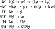
The fundamental composition of the axiomatization system for LTL contains all the tautologies like atomic proposition, Boolean operators in first-order logic. Temporal expressiveness and inference rules are shown as follows:

• A0 All classical tautologies of first-order logic

• A1 □(ϕ→φ)→(□ϕ→□φ)

• A2 ¬○ϕ⇔○¬ϕ

• A3 ○(ϕ→φ)→(○ϕ→○φ)

• A4 □(ϕ→○φ)→(ϕ→□φ)

• A5 (ϕUφ)⇔φ∨○(ϕUφ)

• A6 (ϕUφ)→♢φ

and the inference rules:

• MP $\frac {\phi \quad \phi \rightarrow \varphi }{\varphi }$

• N_□ $\frac {\phi }{\vdash \Box \phi }$

• N_○ $\frac {\phi }{\vdash \bigcirc \phi }$

Gabbay et al. [32] present the completeness of the deductive systems of LTL. Also, Lichtenstein and Pnueli [33] prove the complete system of LTL from three parts: the general part, domain part and program part. The temporal operator next expresses dynamic behaviors in discrete time, so it is unsuitable to express dense time. So the axioms A2-A6 and the inference rule N_○ will be ignored for the axiomatization of STL.

Spatio-temporal specification language

STL provides an approach that combines the truth value and quantitative value of general signals. But it is inadequate to represent the changes of a spatial entity and the binary relation between spatial entities and temporal aspects. We propose the spatio-temporal specification language that combines STL and S4 _u to describe the evolution in spatial and temporal domain.

Spatio-temporal signals

A spatio-temporal signal is defined with continuous time and topometric space [29, 34]. A real-valued interval [0,t) is defined in the dense time domain $\mathbb {T}$, where $t\in \mathbb {R}_{\geq 0}$. Because the time domain inherits STL, it will keep consistency with the interval in STL. The signal function is extended to spatial-temporal domain with $\varepsilon \colon \mathbb {T}\times \mathbb {L} \rightarrow \mathbb {E}$, where $\mathbb {L}$ denotes the topometric space. Firstly, an elementary signal evaluates a spatial entity or the connections between spatial entities. That is, the elementary signal is quantitative signals Secondly, a Boolean signal can be transformed from a quantitative signal by the threshold predicate x_i≥0. The signals stem from topometric space, therefore, the Boolean and quantitative signals are extended from the domain of STL signals to topometric space.

An atomic spatial entity enjoys two meanings: point-based interpretation, point set-based interpretation and region-based interpretation. The points interpret discrete location coordinates. It is consistent with your comment. But, the point set-based interpretation and region-based interpretation denote the discrete and continuous space respectively. When involving in changes of spatial entities, we are talking about motion. The motion of spatial entities can be discrete or dense time. We define a spatio-temporal trace w as the changes of spatial objects over time. Formally, a spatio-temporal trace assigns $\mathbb {T}\times \mathbb {L}$ to a multi-dimensional signal $\mathbb {R}^{n}$, where n refers to the number of variables.

A spatio-temporal trace provides a notation about execution sequence of temporal and spatial domain.

Definition 3.1.

(Spatio-temporal signal) A spatio-temporal signal ε is an evaluation of spatial entities in a trace w. A Boolean signal $\mu _{i}^{w(t)} (i\in \mathbb {N})$ is an evaluation of an atomic proposition transferred from quantitative signals $\mathbf {x}_{i}^{w(t)}$ by atomic predicate $\mu _{i}^{w(t)} = \left (\mathbf {x}_{i}^{w(t)}\geq 0\right)$ in the trace.

$$\varepsilon_{i}^{w(t)} :=\left\{ \begin{aligned} \mu_{i}^{w(t)} \quad if\quad \varepsilon_{i}^{w(t)} \in \mathbb{B}\quad\\ \mathbf{x}_{i}^{w(t)} \quad if\quad \varepsilon_{i}^{w(t)} \in \mathbb{R}_{\geq 0} \end{aligned} \right. $$

where $\mathbb {B}$ refers to the domain of Boolean signals and $\mathbb {R}_{\geq 0}$ quantitative signals.

For a spatio-temporal trace w, there are two different interpretations:

• A trace represents a sequence of spatial objects and time point and each point in the trace evaluates a pair of spatial objects and time.

• Another interpretation means that a spatio-temporal trace takes spatial objects as the basic entities and spatio-temporal primitive relations could be obtained by the changes of ontology of space over time.

In this work, we treat the spatio-temporal trace as the second interpretation. The changes of spatial objects are influenced by the flow of time.

The interpretation of the combined logic

It is essential that a combined spatio-temporal form should be provided with enough expressiveness to contain the three parameters [22]:

• 1 the expressiveness of the spatial component;

• 2 the expressiveness of the temporal component;

• 3 the interaction between the two components allowed in the combined logic.

Based on the principle of PC [22], which expresses that the language should be able to express changes over time of the truth-values of purely spatial propositions. We interpret an STSL _PC formula based on the topometric temporal model, which is defined on topometric space and temporal interval structure in strict partial ordering with a set of sampling time point. The model can be treated as a set of sampling trace monitoring from state-based cyber-physical systems, rather than differential equations [18]. Firstly, the scene snapshot of a system is abstracted to be a topometric model. As the system executes, the system is sampled as a sequence of traces at dense time. At each time instant, the spatial structure denotes a topometric model. And the topometric temporal model in dense time and topometric space can be a sequence of sampling traces. Formally, a topometric temporal model is defined as a triple $\mathfrak {M} = (\mathfrak {T}, \mathfrak {L}, \mathfrak {V})$, where

• $\mathfrak {T}$ is an interval structure $(\mathcal {T}, \mathcal {I}(\mathcal {T}))$, where $\mathcal {T} = (\mathbb {T},<)$ is strict partial ordering with a set of time point $\mathbb {T}$ and < an irreflexive, transitive and asymmetric relation on $\mathbb {T}$ with a linear strict time flow, and $\mathcal {I}(\mathcal {T})$ is a set of intervals,

• $\mathfrak {L}$ is a topometric space with the definition of $(M, \mathbb {I}_{d})$ in which M is a nonempty set, the universe of the space, and $\mathbb {I}_{d}$ is the interior operator on M induced by the metric space (M,d), which satisfies the standard Kuratowski axioms [35]: $\forall X, Y\subseteq M, \mathbb {I}(X\cap Y) = \mathbb {I}X\cap \mathbb {I}Y, \mathbb {I}X\subseteq \mathbb {II}X$ and $\mathbb {I}(M) = M$,

• $\mathfrak {V}$ is a valuation on the time domain $\mathfrak {T}$ and the spatial term set $\mathbb {L}$, i.e., $\forall \tau \in \mathbb {L}$, and $t \in \mathbb {T}$. Formally, $\mathfrak {V}(\tau, t) = \left \{\mu _{i} \mid \forall i\in \mathbb {N}, x_{i}\geq 0\right \}$ means the space occupied by a spatial term τ at time point t. As for the spatial term τ, the valuation can be defined as: $\mathfrak {V}(\overline {\tau }, t) = \neg \mathfrak {V}(\tau, t), \mathfrak {V}(\tau _{1}\sqcap \tau _{2}, t) = \mathfrak {V}(\tau _{1},t)\cap \mathfrak {V}(\tau _{2},t), \mathfrak {V}(\mathbb {I}\tau, t) =\mathbb {I}\mathfrak {V}(\tau,t)$.

The ontology of space includes the static spatial entities and dynamic spatial entities. We describe the ontology of static spatial entities with S4 _u atomic spatial terms and spatial operators like complementary, intersection and union, interior and closure. And the spatial until operator is employed to represent the dynamic spatial ontology. However, the changes of ontology of space means that the evolution of spatial entities can be changed by external event or the arrival of a time slice. The changes of spatial terms in topometric model over time can be shown in Fig. 2.

Fig. 2

The changes of point-based spatial terms over time in topometric model

A topometric temporal model is an abstraction of a cyber-physical system, while a spatio-temporal trace is an execution of topometric temporal model. Generally, classical model checking provides an approach to verify whether a topometric temporal model, i.e., all the traces, satisfies spatio-temporal properties. However, the state space explosion makes it difficult for model checking to verify the reliability and security of real cyber-physical systems. Monitoring verifies whether the spatio-temporal signals on one execution of the system hold the specified spatio-temporal properties. Especially, online monitoring can provide the verification results to help analyze the potential hazards, which can avoid unnecessary loss.

Example 3.1.

One point represents a spatial entity and an edge between two points means the connection between spatial entities. The weight on the edge denotes the metric between spatial entities. At any time instant, the points, edges and weight on the edges consist a undirected weighted graph, which denotes the topological metric models. As time goes, the topometric model leads to the topometric temporal model. In this figure, a spatial term τ is characterized as a 2-dimensional space and the spatial terms change over time in the model $\mathfrak {M}$.

Example 3.2.

The changes of spatial terms in topometric model over time can be shown in Fig. 3. In this figure, a spatial term p is characterized as a 2-dimensional space and the spatial terms change over time in the model $\mathfrak {M}$. The model describes the changes of spatial relations. The y axis describe the spatial relations. In the x axis, the time instant samples the spatial relations between the spatial entities red, blue and green. The black time instants describe the tangential proper part (TPP) relations between three region-based spatial entities green and red. While the red time instants express the partial overlap (PO) relations between green and red. The spatial relations are expressed by S4 _u terms and the spatial relations are sampled with dense time and represented in STL.

Fig. 3

The changes of region-based spatial terms over time in topometric model

Firstly, a cyber-physical system involves in discrete and continuous time. The cyber system describes the execution of an actual system, and the signal is sampled in discrete time. The physical system generally expresses the continuous changes of a spatial entity. A topometric temporal model is an abstract of a cyber-physical system. A spatio-temporal trace is sampled from the topometric temporal model. And the trace is an execution of a cyber-physical system. Further, when the trace describes spatial relations among spatial entities and is sampled in dense time, it will be able to be monitored by STSL formulas.

The concurrency can be interpreted in topometric model. Mainly, we interpret the region through borrowing the notation from Milner’s Bigraph [36], which presents the agent and the communication between different agents. We treat a spatial entity as an agent. Meanwhile, we define the concurrence of topometric model as the concurrency between spatial entities. We present the topometric model in region-based and point-based interpretation. So, we will illustrate the model from two perspectives.

Firstly, the point-based topometric model can consider a list of regions. For instance, S4 _u terms can specify the properties that the region made by spatial entities a₆,a₇ and a₈ exists in the region occupied by the union of the spatial entities a₅,a₆,a₇,a₈ and a₉ as:

$$ \left(a_{6}\sqcup a_{7} \sqcup a_{8}\right)\sqsubseteq \left(a_{5} \sqcup a_{6}\sqcup a_{7} \sqcup a_{8} \sqcup a_{9}\right) $$

(1)

Another properties can be that the spatial entity a₅ belongs to the intersection of the region that made up of spatial entities a₁,a₂,a₃,a₅ and a₆, and the region that made up of spatial entities a₅,a₆,a₇,a₈ and a₉. The property can be specified with S4 _u as:

$$ a_{5} \sqsubseteq \left(a_{1}\sqcup a_{2}\sqcup a_{3} \sqcup a_{5}\sqcup a_{6}\right)\sqcap \left(a_{5}\sqcup a_{6}\sqcup a_{7}\sqcup a_{8} \sqcup a_{9}\right) $$

(2)

From the perspective of agent, the spatial entities are hierarchical, which lead a tree-like structure. The tree-like structure is a place graph in Bigraph. Here, we didn’t define the interfaces or names between spatial entities for communication. Instead, we define the metric between the spatial entities. If we ignore the interfaces or names, the graph in Fig. 4 can be treated as a link graph. The place graph and link graph from topometric model compose the Bigraph. So, the topometric model is able to express concurrency.

Fig. 4

The point-based spatial terms in topometric model

Secondly, region-based topometric model is relatively concise with spatial complementary, intersection, union, interior, closure and until operators. So it is easier to be interpreted. Figure 5 shows the spatial relations between the spatial entities green, red and blue.

Fig. 5

The region-based spatial terms in topometric model

Based on the notation of Bigraph with sharing [37], the overlapping part between two spatial entities can be treated as the sharing part. The hierarchical relations between region-based topometric model are more clear. For instance, we can say that the spatial entity blue and green are concurrent, and their parent spatial entity is concurrent with the red entity.

The spatio-temporal signals are divided into Boolean and quantitative signals. According to the category of spatio-temporal signals, we will present syntax and semantics for the proposed spatio-temporal specification language from two sides:

• The Boolean semantics returns true or false depending on whether the trace of topometric temporal model satisfies the properties or not.

• The quantitative semantics returns a real value in different time that can be interpreted as an evaluation of satisfaction.

The Boolean semantics of the spatio-temporal specification language interprets that an STSL _PC formula over spatio-temporal traces returns true or false, so it is able to express purely spatial propositions’ changes with the truth-values. Meanwhile, the $\mathcal {U}_{I}$ and □_I operators of the quantitative semantics of STSL _PC are able to express satisfaction degree of spatial entities over some fixed finite periods and the whole duration of time, respectively.

The syntax of STSL _PC

As usual, we define the real-value interval in temporal domain. Formally, we confine the temporal interval I to be left-closed right-open $[t, t'), \forall t, t'\in \mathbb {T}$ and t<t^′. The STSL _PC fuses the temporal logic STL and modal spatial logic S4 _u so that the language can express the changes of purely spatial propositions over time. Specifically, the language is defined on spatial terms τ and spatial operators complementary, intersection, union, interior and closure, atomic predicates, Boolean connectives and temporal operators globally, finally and until over the temporal interval I. There are two kinds of atomic predicates: the binary subset operator of two spatial terms $\tau _{1}\sqsubseteq \tau _{2}$ and the threshold predicates on a signal x_i≥0. The spatial subset relation describes the relations between region-based spatial entities. Specifically, the binary subset can be derived by the unary spatial operator universal with the form , where ⊤ denotes the spatial universal set. The quantitative signals evaluate the spatial entities. The Boolean signals can be achieved from the quantitative signals by the threshold predicates. The atomic predicate $\tau _{1}\sqsubseteq \tau _{2}$ means that the elements in the spatial term τ₁ must belong to τ₂. And x_i≥0 is a threshold predicate, which transfers general real-valued signals to Boolean value. The syntax of STSL _PC is given by:

$\tau ::= p \mid \overline {\tau } \mid \tau _{1}\sqcap \tau _{2} \mid \mathbb {I}\tau$

$\varphi ::= \tau _{1}\sqsubseteq \tau _{2} \mid x_{i}\geq 0 \mid \neg \varphi \mid \varphi _{1}\wedge \varphi _{2} \mid \varphi _{1}\mathcal {U}_{I}\varphi _{2}$

• τ is a spatial term,

• p is an atomic spatial variable,

• $\overline {\tau }$ is the complementary of τ,

• τ₁⊓τ₂ is the intersection of τ₁ and τ₂,

• $\mathbb {I}$ is the interior operator under the topometric space interpretation. Moreover, the dual operator of $\mathbb {I}$ is the closure operator $\mathbb {C}$, which means possible or consistent,

• $\tau _{1}\sqsubseteq \tau _{2}$ implies the spatial subset relations, which means that for all points p,p∈τ₁ implies p∈τ₂,

• x_i≥0 is an atomic predicate,

• ¬,∨ and ∧ are the Boolean operators,

• $\mathcal {U}_{I}$ is the until operator.

We can define equivalence of operators as syntactic abbreviations:

$$\begin{aligned} \mathbb{C}\tau &= \overline{\mathbb{I}\overline{\tau}} \\ \tau_{1}\sqcup \tau_{2} &= \overline{\overline{\tau_{1}}\sqcap\overline{\tau_{2}}} \\ \mathbb{I}(\tau_{1}\sqcup\tau_{2}) &= (\mathbb{I}\tau_{1}\sqcup\mathbb{I}\tau_{2}) \\ \mathbb{C}(\tau_{1}\sqcup\tau_{2}) &= (\mathbb{C}\tau_{1}\sqcup\mathbb{C}\tau_{2}) \\ \varphi_{1} \vee \varphi_{2} &= \neg(\neg\varphi_{1} \wedge \neg\varphi_{2}) \\ \Diamond_{I}\varphi &= \top \mathcal{U}_{I}\varphi \\ \Box_{I}\varphi &= \neg\Diamond_{I}\neg\varphi. \end{aligned} $$

Atomic predicates, Boolean operators, and the temporal bounded until operator $\mathcal {U}_{I}$ are from STL. The new spatial operators are the interior operator $\mathbb {I}$ and the closure operator $\mathbb {C}$ with reference to S4 _u. The ♢_I and □_I operators are derived unary operators. □_Iφ denotes that φ holds within the whole interval I, and ♢_Iφ means that φ holds in at least one time point of the interval I.

Example 3.3.

In the mobile blocking mode, the protection point is located behind the forward train to protect the position uncertainty and the back boundary. The protection point is the zero speed limit point, which is a limit that is absolutely not allowed to be crossed by the signal system control. The core of the train’s automatic protection is the safe braking model of the train. It describes how to calculate the emergency braking curve and the normal braking curve of the train in Fig. 6. The emergency braking curve considers the emergency braking deceleration of the train protection, the current protection point calculated by the trackside ATP, the most restrictive speed curve and the slope section of the line. The normal braking curve takes into account the ATP response delay time and the cut-off traction after emergency braking. The ATP on-board computer unit dynamically calculates and continuously monitors the normal braking curve. The safe braking model ensures that the train will not exceed the most restricted speed and the train will stop in front of the protection point. Formally, the location of end of mobility authority is marked with EoA, and that of the end of protection is marked with EoP. The distance from the location of the following train to EoA denotes τ_ma. The distance from the location of the beginning of following train to EoP means τ_p. Also, the braking distance in normal and emergent braking mode is represented as τ_nb and τ_eb. A spatio-temporal property can be expressed as After receiving the signals, the train brakes in the normal braking mode and it keeps running in the region of τ_ma. While the train keeps running without braking in emergent braking model within 10 seconds. After the train brakes in the emergent braking mode, there exists a moment that the velocity of normal braking is larger than that of the emergent braking mode. And the train keeps running in the emergent braking mode in the region of τ_p within 40 seconds. The property can be specified with STSL _PC formula as:

$$ \begin{aligned} &\Box_{[0, 10)}\left(\left(a_{nb}\leq a_{eb}\right)\wedge \left(\tau_{nb}\sqsubseteq\tau_{ma}\right)\right)\wedge \\&\Diamond_{[0,40)}\left(\left(\tau_{eb}\sqsubseteq\tau_{p}\right)\wedge\left(v_{nb}\geq v_{eb}\right)\right) \end{aligned} $$

(3)

Fig. 6

The safety braking model of automatic train protection

where a_nb and a_eb denote the acceleration in normal and emergent braking mode, respectively. v_nb and v_eb represent the velocity in normal and emergent braking mode, respectively.

Example 3.4.

In the example 3.1, we can employ an STSL _PC formula to specify the properties that the region made by spatial entities a₆,a₇ and a₈ exists in the region occupied by the union of the spatial entities a₅,a₆,a₇,a₈ and a₉, until the region made by spatial entities a₃,a₆ and a₈ exists in the region occupied by the union of the spatial entities a₃,a₅,a₆,a₇ and a₈ as

Example 3.5.

In Fig. 3 of example 3.2, we can specify the property that for any execution within 4 seconds, there is an inclusion between two spatial entities τ_blue and τ_grey, and it will follow an overlapping between them within 1.5 seconds. The property can be specified with STSL _PC formula as

(5)

The semantics of STSL _PC

The semantics of STSL _PC is divided into Boolean semantics and quantitative semantics, which return the truth value of purely spatial propositions and real-valued spatial objects. We define μ_i as a predicate because the spatial entities are a discrete set and each signal is evaluated by a threshold predicate μ_i. The quantitative semantics can be transformed to Boolean semantics by a predicate μ_i.

The spatial element of the spatio-temporal specification language exists in spatial entity τ. The value of the spatial entity τ can be achieved by the definition $\mathfrak {V}(\tau, w, t)$. That is, we interpret a spatio-temporal formula in simulated trace rather than topometric temporal model. The satisfaction relation for an STSL _PC formula φ over a topometric temporal model $\mathfrak {M}$ is given by:

• $(w, t)\models \tau _{1}\sqsubseteq \tau _{2} \; \Leftrightarrow \; \mathfrak {V}(\tau _{1}, w, t) \leq \mathfrak {V}(\tau _{2}, w, t)$

• $(w, t)\models x_{i}\geq 0 \; \Leftrightarrow \; \mathfrak {V}(x_{i}, w, t)\geq 0$

• (w,t)⊧¬φ ⇔ (w,t)⊮φ

• (w,t)⊧φ₁∧φ₂ ⇔ (w,t)⊧φ₁ and(w,t)⊧φ₂

• $(w, t)\models \varphi _{1}\mathcal {U}_{I}\varphi _{2} \; \Leftrightarrow \; \exists t'\in t + I \text { s.t.} (w, t') \models \varphi _{2} \text { and} \forall t''\in [t, t'], (w, t'')\models \varphi _{1}$

A trace w satisfies an STSL _PC formula φ at t, denoted by (w,t)⊧φ. For the satisfaction relation, the “ ⇒” answers whether the implementation procedure of computation holds the specification relation. The “ ⇐” can be achieved from the definition of satisfaction relation of an STSL _PC formula φ.

For a given formula φ and execution trace w, we define the satisfaction signal χ(φ,w,t) over a trace w(t,l):

$$ \forall t\in I,\; \chi(\varphi,w, t) := \left\{ \begin{aligned} \top \; \text{ if}\ (w,t)\models \varphi\\ \bot \quad\; \mathbf{otherwise}\;\;\; \end{aligned} \right. $$

(6)

where ⊤ and ⊥ respectively denote Boolean value true and false. Therefore, $\chi (\tau _{1}\sqsubseteq \tau _{2}, w, t)$ returns true if spatial subset relation $\tau _{1}\sqsubseteq \tau _{2}$ holds over the model. For a general signal x_i,χ(x_i,w,t) returns true if x_i≥0 in the trace w(t). χ(□_Iφ,w,t) means that for all t∈I,φ always returns trues in the interval I over the model. While χ(♢_Iφ,w,t) denotes that there exists t∈I,φ returns trues in the interval I over the model.

In order to compute the satisfaction of a formula φ, we divide the formula φ into each subformula ϕ_i until atomic formula so that formula φ can be computed through the subformula and atomic formulas instead of the entire satisfaction signal χ(φ,w,t). The procedure can be treated as a hierarchical structure from the full formula φ down to each atomic formula.

We define ρ to quantify the satisfaction degree of the property φ over the trace w(t), and it returns a real value ρ(φ,w,t). For an atomic spatial formula , the satisfaction degree can be evaluated as $\mathcal {V}(\tau, w, t)$. And for a atomic predicate x_i≥0 can be evaluated as $x_{i}^{w(t)}$. The quantitative satisfaction relation for a formula φ over a spatio-temporal trace w at the time t by the notation of satisfaction degree is given by:

• .

• $\rho (x_{i} \geq 0, w, t) \; = \; x_{i}^{w(t)}$

• ρ(¬φ,w,t) = −ρ(φ,w,t)

• ρ(φ₁∧φ₂,w,t) = min{ρ(φ₁,w,t),ρ(φ₂,w,t)}

• ρ(φ₁∨φ₂,w,t) = max{ρ(φ₁,w,t),ρ(φ₂,w,t)}

• ρ(□_Iφ,w,t) = inft^′∈t+I{ρ(φ,w,t^′)}

• ρ(♢_Iφ,w,t) = supt^′∈t+I{ρ(φ,w,t^′)}

• $\rho (\varphi _{1} \mathcal {U}_{I}\varphi _{2}, w, t) = \sup _{t'\in t + I}(\min \{\rho (\varphi _{2}, w, t'), \inf _{t''\in [t,t']}(\rho (\varphi _{1}, w, t'')\})$

The negation of a formula is evaluated as the negative of its satisfaction degree. The conjunction and disjunction of two formulas are evaluated as the minimum and maximum of the satisfaction degree of the two formulas. ρ(□_Iφ,w,t) refers to that the infimum of ρ(φ,w,t^′),∀t^′∈t+I is always true in the interval I over the trace. Similar to ρ(□_Iφ,w,t),ρ(♢_Iφ,w,t) returns the truth value of the supremum of ρ(φ,w,t^′),∀t^′∈t+I. The satisfaction degree of until formula $\varphi _{1} \mathcal {U}_{I}\varphi _{2}$ is evaluated complexly. Firstly, we achieve the satisfaction degree of the formula φ₂ in the time t^′, which belongs to the interval t+I. Secondly, the infimum of the formula φ₁ is evaluated in the interval of [t,t^′). Thirdly, the minimum of the result of first steps is achieved. At last, the satisfaction degree of until formula $\varphi _{1} \mathcal {U}_{I}\varphi _{2}$ is evaluated as supremum of the minimum in the third step. It is worthy noting that the infimum of the satisfaction degree of a formula means that the minimum value of the signals within temporal interval I. Similarly, the supremum of the satisfaction degree of a formula denotes the maximum value of signals with a temporal interval I.

The connection between Boolean and quantitative signals is built by the way of predicate x_i≥0 and obtain the satisfaction signal χ(x_i≥0,w,t), which returns a real value of the quantitative signals x_i representing the distance to satisfaction. Specifically, the satisfaction degree of quantitative signal can be derived from the Lemire’s algorithm [38] through MAX-MIN filter of a running sequence.

Example 3.6.

In Fig. 3, we can specify the property that for any execution within 4 seconds, there is an inclusion between two spatial entities τ_blue and τ_grey, and it will follow an overlapping between them within 1.5 seconds. The property can be specified as

(7)

Completeness and decidability of STSL _PC

The language STSL _PC describes the spatial changes in dense time, which is used to monitor the execution of continuous systems at run time. So we ignore the temporal next operator that describes the next step of the discrete systems.

An axiomatization system of STSL _PC

We will present a Hilbert-style proof system for STSL _PC according to expressiveness of the proposed language. STSL _PC combines temporal logic and spatial logic, so the proof system will be introduced from spatial and temporal part. Further, the temporal operators □_I,♢_I and $\mathcal {U}_{I}$ are defined in an interval I in dense time, so we will add the quantitative part for the proof systems.

Spatial part

The spatial part of the axiomatization presents the subset relation of spatial terms with complementary, intersection and union operators:

• S0 $\mathbb {I}\tau \sqsubseteq \tau$

• S1 $\tau \sqsubseteq \mathbb {C}\tau$

• S2 $\tau _{1}\sqsubseteq \tau _{2} \leftrightarrow \overline {\tau _{2}}\sqsubseteq \overline {\tau _{1}}$

• S3 $\tau _{1}\sqsubseteq \tau _{2} \leftrightarrow \mathbb {C}\tau _{1}\sqsubseteq \tau _{2}$

• S4 $\tau _{1}\sqsubseteq \tau _{2} \leftrightarrow \tau _{1}\sqsubseteq \mathbb {I}\tau _{2}$

• S5 $\tau _{1}\sqsubseteq \tau _{2} \leftrightarrow \mathbb {I}\tau _{1}\sqsubseteq \mathbb {I}\tau _{2}$

• S6 $\tau _{1}\sqsubseteq \tau _{2} \leftrightarrow \mathbb {C}\tau _{1}\sqsubseteq \mathbb {C}\tau _{2}$

• S7 $\tau _{1}\sqsubseteq \mathbb {I}\tau _{2}\rightarrow \tau _{1}\sqsubseteq \mathbb {C}\tau _{2}$

• S8 $(\tau _{1}\sqcup \tau _{2})\sqsubseteq \tau _{3}\rightarrow (\tau _{1}\sqsubseteq \tau _{3})\vee (\tau _{2}\sqsubseteq \tau _{3})$

• S9 $\tau _{1}\sqsubseteq (\tau _{2}\sqcap \tau _{3})\rightarrow (\tau _{1}\sqsubseteq \tau _{2})\wedge (\tau _{1}\sqsubseteq \tau _{3})$

• S10
• S11
• S12

And the inference rules:

• $N_{\sqsubseteq }$ $\frac {\tau _{1}\sqsubseteq \tau _{2} \quad \tau _{2}\sqsubseteq \tau _{3}}{\vdash \tau _{1}\sqsubseteq \tau _{3}}$

Temporal part

The temporal part of STSL _PC in real time with interval implies that the temporal next operator is forbidden.

• T0 All classical tautologies of propositional logic

• T1 ♢_Iϕ⇔¬□_I¬ϕ

• T2 □_I(ϕ∧φ)→(□_Iϕ∧□_Iφ)

• T3 ♢_I(ϕ∨φ)→(♢_Iϕ∨♢_Iφ)

• T4 ϕU_Iφ→♢_Iφ

And the inference rules:

• MP $\frac {\phi \quad \phi \rightarrow \varphi }{\varphi }$

• N_□ $\frac {\phi }{\vdash \Box _{I}\phi }$

Axiom (T0) and Modus Ponens (MP) are from the Hilbert-style axiomatization of propositional logic. Axioms (T1-T4) are achieved from by Manna and Pnueli’s temporal logic [39]. A complete proof system for quantitative version is proposed in [40].

Quantitative part

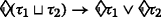
The quantitative part of spatio-temporal logic involves the execution of system in dense time, so the quantitative axioms need to be provided. We follow the way of [41] to present the quantitative axioms for STSL _PC. However, we forbid the appearance of the punctuality in interval as the metric logic MITL and ban the temporal next operator because of the continuous time. The quantitative axioms characterize the translation from the intersection, union of intervals into conjunction, disjunction of temporal operators with interval. Specifically, the intersection of two intervals is bounded in finally operator with the form ♢_I∪Jφ, and it implies the disjunction of finally operator bounded with their respective interval. Conversely, the disjunction of finally operator bounded with their respective interval implies the finally operator bounded with the union of the two intervals. However, the globally operator bounded with the intersection of the two intervals and the conjunction of globally operator bounded with their respective interval imply each other. For until operator, the axiom generalizes ϕU_Iφ→♢_Iφ with the union of two intervals I∪J.

• Q0 ♢_I∪Jφ⇔♢_Iφ∨♢_Jφ

• Q1 □_I∩Jφ⇔□_Iφ∧□_Jφ

• Q2 ϕU_I∪Jφ→♢_I∪Jφ

Soundness and completeness of the axiomatization system

Once an axiomatization system is present, the soundness and completeness of the axiomatization system need to be proved, including spatial, temporal and quantitative axioms. Soundness refers to that all the theorems in STSL _PC are logically valid. Equivalently, a spatio-temporal logic is sound with respect to topometric temporal model if for all the formulas $\phi, \vdash _{\mathcal {ST}\phi }$ implies $\Vdash \phi$. Let $\mathcal {ST}$ be a class of topometric temporal modelred. A spatio-temporal logic is strongly complete in $\mathcal {ST}$ if for any set of formulas Γ∪{ϕ}, if $\Gamma \Vdash _{\mathcal {ST}} \phi$ then $\Gamma \vdash _{\mathcal {ST}}\phi$. If the semantics of Γ satisfies ϕ on $\mathcal {ST}$ then ϕ is deducible from Γ.

Theorem 4.1.

The above axiomatization is sound for topometric temporal model, i.e., for any ϕ∈STSL_PC, if ⊩_Γϕ implies $\Vdash _{\mathcal {ST}}\phi$

Proof

The soundness theorem proof need guarantee each axiom is sound and the inference rules preserve soundness from the sound hypothesis. This follows the fact that all axioms are valid and all rules preserve validity. We provide the proof in Appendix A. □

It is well-known that weak completeness plus compactness implies strong completeness [42]. The lexicographic products of modal logic with linear temporal logic are sound and complete [43]. MTL, which empowers more expressiveness in punctuality operator than MITL, is complete in two-sorted model [44]. But temporal logic in the flow of real time has weak completeness [45], which proposes finitely complete and expressively complete, but fails compactness theorem. These conclusions contribute to the result of weak completeness.

Theorem 4.2.

The system for STSL _PC is weakly complete with respect to topometric temporal model, i.e., for every STSL _PC formulas, $\Vdash _{\mathcal {ST}}\phi$ implies ⊩_Γϕ.

Before presenting the complete proof of the axiomatization system of STSL _PC, we will introduce the notation of maximal consistent set [46].

The axiomatization system of STSL _PC is a logical system. A proof in STSL _PC is a sequence of finite formula: A₀,A₁,...,A_n, where each of them is an axiom, or there exists j,k<i, such that A_i is the conclusion derived from A_j and A_k using MP inference rule. The last term A_n is a theorem in STSL _PC, using the sign ⊩A_n, where n is the length of proof.

The concepts of deducibility and consistency from [12, 47] are fundamental to deduce the logic system STSL _PC. A formula A is deducible from a set of formulas Γ in a system $\mathcal {ST}$, written $\Gamma \Vdash _{\mathcal {ST}}A$, if and only if $\mathcal {ST}$ contains a theorem of the form (A₁∧...∧A_n)→A, where the conjunctions A_i(i=1,...,n) of the antecedent are formulas in Γ. A set of formulas Γ is consistent in $\mathcal {ST}$, written ${Con}_{\mathcal {ST}}\Gamma$, just in case the formula ⊥ is not $\mathcal {ST}$-deducible from Γ.

Definition 4.1.

($\mathcal {ST}$-MCS) A set of formulas Γ is maximal $\mathcal {ST}$-consistent iff

• (i) Γ is $\mathcal {ST}$-consistent, and

• (ii) for every formula A, if Γ∪{A} is $\mathcal {ST}$-consistent, then A∈Γ.

If Γ is a maximal $\mathcal {ST}$-consistent set of formulas then we say it is an $\mathcal {ST}$-MCS. The (ii) condition refers to that any set of formulas properly containing Γ is $\mathcal {ST}$-inconsistent.

The canonical model is defined in [47] to induce the soundness and completeness of modal logics. We extend the notation of canonical model to spatio-temporal systems for completeness of STSL _PC.

Definition 4.2.

($\mathcal {ST}$-canonical Model) The $\mathcal {ST}$-canonical model $\mathfrak {M}^{\Gamma }$ for a spatio-temporal logic is a triple (W^Γ,R^Γ,V^Γ) where:

• (i) W^Γ is the set of all Γ-MCSs;

• (ii) R^Γ is the metric relation on topometric space over a quasi-order on time. It is the canonical binary relation on W^Γ defined by $s R_{i}^{\Gamma }s'$ over state s and s^′ if for all formulas ϕ,ϕ∈s implies ϕ∈s^′.

• (iii) V^Γ is the valuation defined by V^Γ(p)={s∈W^Γ∣p∈s}. V^Γ is called the canonical valuation.

Lemma 4.3.

(Truth Lemma) Let $\mathcal {ST}$-canonical model be a class of topometric temporal model. For all $\phi \in \mathcal {ST}$-MCS, $\mathcal {ST}\Vdash \phi$ iff $\phi \in \mathcal {ST}$-MCS.

Proof

The proof is by induction on the structure of ϕ.

Base case: Suppose ϕ is a spatial formula or an atomic predicate x_i≥0.

$(\mathcal {ST}, s)$ ,

$(\mathcal {ST}, s)\Vdash x_{i}\geq 0 \Leftrightarrow V^{\Gamma }(x_{i}\geq 0,s)=x_{i} \Leftrightarrow x_{i}\geq 0\in s$.

Inductive step: Suppose ϕ is an atomic predicate $\neg \phi, \phi _{1}\wedge \phi _{2}, \phi _{1}\vee \phi _{2}, \Box _{I}\phi, \Diamond _{I}\phi, \phi \mathcal {U}_{I}\varphi$. We show the proof of the case □_Iϕ, and leave the others to reader. We have $(\mathcal {ST}, s)\Vdash \Box _{I}\phi \Leftrightarrow \Box _{I}\phi \in s$ (assuming the inductive hypothesis).

$(\mathcal {ST}, s)\Vdash \Box _{I}\phi$

$\Leftrightarrow \forall s', sR^{\Gamma }s'\Rightarrow \mathcal {ST}, s'\Vdash \phi$

⇔∀,sR^Γs^′⇒ϕ∈s^′

we need to show that □_Iϕ∈s⇔∀s^′,sR^Γs^′⇒ϕ∈s^′.

⇒ follows immediately from the Definition 4.2.

As for ⇐: suppose □_Iϕ∉s. We need to show

∃s^′,sR^Γs^′ and ϕ∉s^′

⇔∃s^′,sR^Γs^′ and ¬ϕ∈s^′

⇔∃s^′,{φ∣□_Iφ∈s}⊆s^′ and ¬ϕ∈s^′

⇔∃s^′,{φ∣□_Iφ∈s}∪{¬ϕ}⊆s^′

It is easy to show that {φ∣□_Iφ∈s}∪{¬ϕ} is $\mathcal {ST}$-consistent. Suppose not, i.e., {φ∣□_Iφ∈s}∪{¬ϕ} is $\mathcal {ST}$-inconsistent. Then $\vdash _{\mathcal {ST}}(\varphi _{1}\wedge...\wedge \varphi _{n})\rightarrow \phi$ for some {□_Iφ₁,...□_Iφ_n}⊆s. But $\mathcal {ST}$ is canonical and s is $\mathcal {ST}$-MCS, so s must contain (□_Iφ₁∧...∧φ_n)→□_Iϕ. From □_Iφ_i∈s, it follows □_Iϕ∈s. This contradicts the hypothesis that □_Iϕ∉s □

The proof of the weakly complete system of STSL _PC is immediately the result of Lemma 4.3.

Decidability of of STSL _PC

We present the decidability of STSL _PC based on the finite model property [12]. A decision procedure for the decidable fragment will be present.

Definition 4.3.

(Filtration) Let $\mathfrak {M}$ be the topometric temporal model and φ subformula closed set of formulas. ≈ is an equivalence relation on the states of $\mathfrak {M}$ defined by:

(t,l)≈(t^′,l^′) iff for all ϕ in φ: $(\mathfrak {M},t,l)\Vdash \phi$ iff $(\mathfrak {M},t',l')\Vdash \phi$.

We denote the equivalence class of a state with respect to ≈ by |(t,l)|. Let $(\mathbb {T},\mathrm {U})=\{|(t,l)|\mid (t,l)\in (\mathbb {T},\mathrm {U})\}$. Suppose $\mathfrak {M}^{f}$ is any model $(\mathfrak {T}^{f}, \mathfrak {L}^{f}, \mathfrak {V}^{f})$ such that:

• $(\mathfrak {T}^{f},\mathfrak {L}^{f})=(\mathfrak {T}, \mathfrak {L})$.

• if (t,l)≈(t^f,l^f) then |(t,l)|≈|(t^f,l^f)|.

• if |(t,l)|≈|(t^f,l^f)| then for all ♢ϕ∈φ, if $(\mathfrak {M},t,l)\Vdash \phi$ then $(\mathfrak {M},t',l')\Vdash \Diamond \phi$.

• $\mathfrak {V}^{f}(p)=\{|(t,l)|\mid (\mathfrak {M},t,l)\Vdash p\}$ for all proposition letters p in φ.

Then $\mathfrak {M}^{f}$ is a filtration of $\mathfrak {M}$ through φ.

Proposition 4.1.

Let φ subformula closed set of STSL _PC formulas. For any model $\mathfrak {M}$ if $\mathfrak {M}^{f}$ is a filtration of $\mathfrak {M}$ through a subformula closed set φ, then $\mathfrak {M}^{f}$ contains at most 2ⁿ nodes (where n denotes the size of φ).

Theorem 4.4.

(Filtration Theorem) Let $\mathfrak {M}^{f} = (\mathfrak {T}^{f}, \mathfrak {L}^{f}, \mathfrak {V}^{f})$ be a filtration of $\mathfrak {M}$ through a subformula closed set φ. Then for all formulas ϕ∈φ, and all nodes (t,l) in $\mathfrak {M}$, we have $(\mathfrak {M},t,l)\Vdash \phi$ iff $(\mathfrak {M}^{f},|(t,l)|)\Vdash \phi$

Theorem 4.5.

(Finite Model Property) If ϕ is satisfiable, then it is satisfiable on a finite model. Indeed, it is satisfiable on a finite model containing at most zⁿ, where n is the number of subformulas of ϕ.

Proof

If ϕ is satisfiable in the filtration is immediate from Theorem 4.4, and the bound od size of the filtration is immediate from Proposition 4.1. It is well-known in standard case [12, 16]. □

The satisfiability means for all STSL _PC formula ϕ there is a spatio-temporal trace in topometric temporal model $\mathfrak {M}$ such that $(\mathfrak {M}, t,l)\Vdash \phi$. Theorem 4.5 shows the searching is finite in the nodes of topometric temporal model. So it follows Theorem 4.6.

Theorem 4.6.

The satisfiability problem for STSL _PC against topometric temporal model is decidable.

Further, we have the complexity of the decidable STSL _PC.

Theorem 4.7.

The satisfiability problem for STSL _PC against topometric temporal models $\mathfrak {M}$ based on $(\mathbb {N},<), (\mathbb {Z}, <)$ is EXPSPACE-complete.

Proof

Recall that STSL _PC refers to the changes over time of truth-values of purely spatial propositions. The interaction between spatial and temporal components of STSL _PC is very restricted to the elementary unit: purely spatial propositions. The proof will be carried through construction step, reduction step and a decision procedure.

Construction step: For every STSL _PC-formula φ, one can construct an STL-formula ϕ by replacing every occurrence of a spatial proposition $\tau _{1}\sqsubseteq \tau _{2}$ and atomic predicate x_i≥0 in φ with a fresh propositional variable. Specifically, given an STL-model $\mathfrak {M} = (\mathfrak {T},\mathfrak {V})$ and an STL-formula ϕ with a time point t in $\mathfrak {T}$, we construct the set

$\phi _{t} = \{ \tau _{1}\sqsubseteq \tau _{2}\mid (\mathfrak {M},t)\models \varphi \}\cup \{ x_{i}\geq 0\mid (\mathfrak {M},t)\models \varphi \}$.

of spatial formulas as a collection of STL proposition variables. If ϕ_t is satisfiable for every t in $\mathfrak {T}$, then there is a topometric temporal model $\mathfrak {M}$ satisfying φ and based on the flow $\mathfrak {T}$.

Reduction step: Definitely, one can obtain the formulas □_Iφ and ♢_Iφ from φ₁U_Iφ₂, so checking whether an STL formula ϕ is satisfiable or not depends on the complexity of computing a formula with U_I operators. In fact, the time domain of STL is bound in the interval I, and an STL formula in Boolean signal returns true or false for a given STL model $\mathfrak {M}$. The bound STL only with Boolean value has the same expressiveness with MITL [29]. It suffices to reduce the satisfiability problem of STL to the satisfiability problem for MITL [48] over infinite trace with interval to check satisfiability of ϕ_t. Further, STL is interpreted in a temporal trace, while MITL is interpreted in timed automata, which capture all trace. The Boolean semantics of STL returns Boolean value, which is equal to MITL. However, STL can be interpreted in quantitative semantics, which returns real value. It makes STL enjoy more powerful expressiveness. STL and MITL have the same expressiveness in temporal interval because the interval in both of them is dense time.

Decision Procedure: We divide the procedure for deciding the satisfiability of STSL _PC into two steps: the first is deciding spatial formula ϕ_t in PC, the second is dealing with STL. According to the observation [29], an STL formula in Boolean semantics is as expressive as an MITL formula, so an Satisfiability Modulo Theories (SMT) [49]-based decision procedure for an MITL is suitable to decide an STL formula in Boolean semantics. We present a decision procedure to satisfiability checking of MITL, which is similar to the approach in [50]. The difference is that we restrict our MITL formula without past tense and the counting modality. We propose the encoding of MITL to Constraint LTL over clock (CLTLoc) [51], which is an extension of Constraint LTL [52] with clocks. □

Lemma 4.8.

([50]) Let M be a signal, and ϕ be an MITL formula. For any (π,σ)∈r_sub(ϕ)(M), we have $(\pi,\sigma),0\models \bigwedge _{\theta \in sub(\phi)}{ck}_{\theta } \wedge \bigwedge _{\theta =F_{(a,b)}(\gamma)} {auxck}_{\theta }$ and for all $k\in \mathbb {N}, \theta \in sub(\phi)$, we have (π,σ),k⊧m(θ).Conversely, if $(\pi,\sigma),0\models \bigwedge _{\theta \in sub(\phi)}({ck}_{\theta }\wedge G(m(\theta))) \wedge \bigwedge _{\theta =F_{(a,b)}(\gamma)} {auxck}_{\theta }$, then there is a signal M such that (π,σ)∈r_sub(ϕ)(M).

The proof can be found in [50]. Let θ be the subformula of MITL formula ϕ, then θ is one of the form $\neg \phi, \phi \wedge \varphi, \phi \mathcal {U}_{I}\varphi, \Diamond _{I}\phi$. The function m(θ) is defined to describe the translation of subformula θ of an MITL formula to a corresponding CLTLoc formula, which is the form:

$$ {init}_{\theta} \bigwedge_{\theta\in sub(\phi)}({ck}_{\theta}\wedge G(m(\theta))) \wedge \bigwedge_{\theta=F_{(a,b)}(\gamma)} {auxck}_{\theta} $$

(8)

The transformation from MITL to CLTLoc is implemented by qtlsolver [53]. The decision procedure of the CLTLoc formula is described in [54], which relies on the Zot toolkit [53]. In [50], it shows the satisfiability of an CLTLoc formula is PSPACE in the size of the formula and in the binary encoding of the constants, the decision procedure induced the encoding is in EXPSPACE.

STSL _OC

The interaction between the spatial and temporal components should comply with the principle of PC and OC [22], which is used to evaluate the interaction:

• STSL _PC: the language should be able to express changes over time of the truth-values of purely spatial propositions.

• STSL _OC: the language should be able to express changes or evolution of spatial objects over time.

STSL _PC expresses the change of truth-value of proposition and it is the elementary requirement for a combined spatio-temporal logic. For STSL _OC, spatio-temporal properties are specified about the changes of spatial objects over dense time with interval through extending the temporal globally, eventually, until operators to spatial terms of STSL _PC. The spatio-temporal trace comply the finite variability. The trace are divided into some intervals. The STSL _OC formulas with these intervals are also verified at runtime.

The difference between STSL _PC and STSL _OC exists that STSL _PC involves in the change of truth-values of propositions, while STSL _OC describes the change of extensions of predicates. Specifically, STSL _PC expresses static spatial terms in topometric space over dense time through spatial complementary, intersection and union operators. The dynamic evolution of STSL _OC is achieved by admitting spatial until operators with interval [l₁,l₂) to spatial terms in topometric temporal model.

The spatial until $\tau _{1}\mathcal {U}_{[l_{1},l_{2})}\tau _{2}$ at spatial location l₁ consists of those points x of the topometric space for which there is l₂>l₁ such that x belongs to τ₂ at moment l₂ and x is in τ₁ at all l whenever l₁<l<l₂. The difference between spatial until and temporal until exists in that spatial until is interpreted as spatial interval [l₁,l₂), and temporal until is defined in a temporal interval [t₁,t₂). Further, spatial until operates two spatial terms τ₁ and τ₂, while temporal until operates two formulas φ₁ and φ₂. The syntax of STSL _OC is given by:

$\tau ::= p \mid \overline {\tau } \mid \tau _{1}\sqcap \tau _{2} \mid \mathbb {I}\tau \mid \tau _{1}\mathcal {U}_{[l_{1},l_{2})}\tau _{2}$

$\varphi ::= \tau _{1}\sqsubseteq \tau _{2} \mid x_{i}\geq 0 \mid \neg \varphi \mid \varphi _{1}\wedge \varphi _{2} \mid \varphi _{1}\mathcal {U}_{[t_{1},t_{2})}\varphi _{2}$

Similar to the atomic formulas, the unary operators □_I and ♢ of spatio-temporal term can also be derived from the operator $\mathcal {U}_{I}$. The occupied spaces of term □_Iτ and ♢_Iτ at moment w are interpreted as the intersection and union of all spatial extensions of τ at moments v>w, respectively.

Example 5.1.

In the Example 3.3, what we can also guarantee is that After the train brakes in the emergent braking mode, there exists a moment that the velocity of normal braking is larger than that of the emergent braking mode within 40 s. And the train keeps running in the normal braking mode in the region of τ_nb until it runs in the region of τ_eb within the spatial interval [p_nb,EoA). The specification can be expressed as

(9)

where v_eb and v_nb mean the velocity of the emergent and normal braking mode.

Example 5.2.

The railway traffic with sensors, present by Liu et.al [2], provides a good perspective to discuss the proposed spatio-temporal specification language. In their example, a train and a control zone can be treated as a region-based spatial terms. Obviously, the spatial region of control zone seems bigger than the region of train. Therefore, the spatial relation between control zone and the train can be characterized as S4 _u formulas or RCC-8 relations, i.e., disconnected (DC), externally connected (EC), partial overlap (PO), equal (EQ), tangential proper part (TPP) and tangential proper part inverse (TPPI), and non-tangential proper part (NTPP) and nontangential proper part inverse (NTPPI). The changes of spatial relations over dense time can be specified by STSL _PC. The specification a train intersects with the control zone until the train leaves within 10 min can be expressed as

$$ PO(\tau_{train},\tau_{cz})\mathcal{U}_{[0,10)}DC(\tau_{train},\tau_{cz}) $$

(10)

where τ_cz means the region of control zone. The predicate PO(τ_train,τ_cz) is equal to the STSL _PC formula (Iτ_train⊓Iτ_cz∧¬ $(\tau _{train}\sqsubseteq \tau _{cz})\wedge \neg$ $(\tau _{cz}\sqsubseteq \tau _{train})$, and the predicate DC(τ_train,τ_cz) can be expressed by the STSL _PC formula .

However, it is not enough to specify spatio-temporal properties with STSL _OC because there is no evolution of spatial entities. Further, it can not even be specified with the spatial relation between point-based spatial terms in topometric space.

Example 5.3.

In example 3.1, the spatio-temporal properties that the spatial entity a₁ reaches a₉ within 20, until the distance from the spatial entity a₁ to a₉ is reduced 18 within 8 min can be specified with STSL _OC as

(11)

The production of temporal logic and spatial logic expresses the spatial evolution in real time with spatial until. The axioms for STSL _OC will add the spatial until. The added operator has no influence on STSL _OC. So the STSL _OC enjoys the same soundness as STSL _PC.

Theorem 5.1.

STSL _OC isn’t complete with respect to topometric temporal model.

Proof

The incomplete STSL _OC can be proved by the counter example: $\Box _{I}(\Diamond _{I}(\tau _{1}\sqcup \tau _{2})\sqsubseteq \Diamond _{I}\tau _{1}\sqcup \Diamond _{I}\tau _{2})\rightarrow \Box _{I}\Diamond _{I}(\tau _{1}\sqcup \tau _{2})\sqsubseteq \Box _{I}(\Diamond _{I}\tau _{1}\sqcup \Diamond _{I}\tau _{2})$. Although the axioms T2 can be applied into temporal deduction, the formula □_I on the spatial terms returns the quantitative space. □

A spatio-temporal trace w is a sequence over signals ε. The Boolean satisfaction relation and satisfaction degree for an STSL _OC formula φ over a spatio-temporal trace w are similar to that of STSL _PC formula.

The decidability of STSL _OC will follow:

Theorem 5.2.

The satisfiability problem for STSL _OC formulas based on $(\mathbb {N},<), (\mathbb {Z}, <)$ is undecidable.

Before providing the proof of Theorem 5.2, we present the lemma 5.3:

Lemma 5.3.

There exists a natural number $\mathbb {N}\geq 1$ and a sequence i₁,...,i_N of indices such that $v_{i_{1}},...,v_{i_{N}}= w_{i_{1}},...,w_{i_{N}}$, then the satisfiability problem for STSL _OC formulas based on $(\mathbb {N},<), (\mathbb {Z}, <)$ is undecidable.

Proof

As we all know, Post’s correspondence problem is undecidable [55]. Given a finite alphabet A={a₁,...,a_m} and a finite set P of pairs (v₁,w₁),...,(v_k,w_k) of nonempty finite sequences (words) v_i,w_i over A, decide whether there exists an N≥1 and a sequence i₁,...,i_N of indices such that $v_{i_{1}},...,v_{i_{N}}= w_{i_{1}},...,w_{i_{N}}$.

An execution trace w is a set of STL signals $\left \{x_{1}^{w},..., x_{k}^{w}\right \}$ defined over some interval D of $\mathbb {R}^{+}$ [11]. Assume the real-valued signals are finite variability. The interval $[t_{i}, t_{i+1})_{i\in \mathbb {N}}$ and threshold predicates divide the execution trace to be piecewise Boolean signals.

We encode the satisfiability problem of STSL _OC formulas to Post’s correspondence problem as the way of [22]. The decidability with less expressive language initially is proved in [56]. We construct a formula φ_A,P which is STSL _OC-satisfiable iff for each 1≤i≤k, let l_i and r_i be the length of words v_i and w_i, respectively, and let

$$\begin{aligned} v_{i} = \left(b_{0}^{i},...,b_{l_{i}}^{i}\right),\\ w_{i} = \left(c_{0}^{i},...,c_{l_{i}}^{i}\right). \end{aligned} $$

The formula φ_A,P is construct as:

$$\varphi_{A,P} = \varphi_{range}\wedge\varphi_{stripe}\wedge\varphi_{pair}\wedge\varphi_{eq}\wedge\varphi_{left}\wedge\varphi_{right} $$

where

φ_range=range∧♢_I¬range∧□_I(¬range→□_I¬range)

$\varphi _{pair} = \Box _{I}(\Diamond _{I} range\rightarrow \bigvee _{1\leq i \leq k} {pair}_{i} \wedge \bigwedge _{1\leq i< j\leq k} \neg ({pair}_{i}\wedge {pair}_{j}))$

φ_stripe=□_I $(stripe \sqsubseteq \Box stripe)\wedge \Box _{I}$ $(\overline {stripe}\sqsubseteq \Box \overline {stripe}))$

$\varphi _{eq} = \Diamond _{I}(range \wedge \bigwedge _{a\in A}$ (left_a≡left_b))

where left_a and right_a(a∈A), left, right and stripe are spatial variables, for every pair (v_i,w_i)(1≤i≤k),pair_i are propositional variables. The variable range is required to ‘relativise’ temporal operators □_I and ♢_I in order to ensure that we can construct a model based on a finite flow of time.

ψ_left is a conjunction of (12)-(18), for all i in 1≤i≤k, and for all j<l_i,

(12)

(13)

(14)

(15)

(16)

(17)

(18)

The conjunct ψ_right is defined by replacing in ψ_left all occurrences of left with right, left _a with right _a (for a∈A) l_i with r_i and the sequence of $left_{b_{j}^{i}}$(for 1≤j≤l_i) with $right_{c_{j}^{i}}$(for 1≤j≤r_i). (Note that pair _i occurs in both ψ_left and ψ_right.)

Because of the difference between spatio-temporal logics and the corresponding model from [57], we change the Aleksandrov tt-model $\mathfrak {M} = ((\mathbb {N},<), \mathfrak {G},\mathfrak {V})$ with $\mathfrak {G} = (V,R)$ to topometric temporal model $\mathfrak {M} = (\mathfrak {T}, \mathfrak {L}, \mathfrak {V})$ with $\mathfrak {L} = (M,\mathbb {I}_{d})$.

Since stripe holds in $\mathfrak {M}$ at 0, we have, for every $y\in M, \mathfrak {M}, (0,y)\models stripe$ iff $\mathfrak {M}, (j,y)\models stripe$ for all j, 1≤j≤N. The transitive binary relation R_s on V defined by taking xR_sy will be modified to the distance relation d on the topometric space M defined by taking d(x,y). The condition will be changed to that if there is z∈M such that ∃ε,d(x,z)<ε and d(z,y)<ε, and (M,(0,x))⊧stripe holds iff (M,(0,z))⊮stripe. □

Theorem 5.2 is the immediate result of Lemma 5.3.

Case study

The example of the train collision avoidance system can be treated as a cyber-physical system. In cyber system, the electrical signals are discrete, and the system clock ticks discretely. However, in physical environment, the running of the train follows kinetic equation, which is continuously changing. The execution of the train collision avoidance system is characterized a sequence of trace, which describes the evolution of spatial region.

The region of movement authority is defined as a special rail sections from the position that an train is authorized to enter to the end of movement authority (EoA), which is the position that the train reaches the safety margin of the leading train. A train must send a movement authority request and receive a permission before the train can enter the next section. In case of emergency, the following train must brake without the permission. In Fig. 7, $p_{ma\_req}$ and p_brake refer to the position that the following train sends a movement authority request and the braking position, respectively. The braking distance τ_bd occupies the section from the braking position p_brake to EoA. If the region of movement authority τ_ma is treated as the universal set, we can describe the spatial relation as

$$ \tau_{bd}\sqsubseteq\tau_{ma} $$

(19)

Fig. 7

The speed-distance curve of mobility authority

And $\overline {\tau _{bd}}$ refers to the distance that the movement authority τ_ma minus the braking distance τ_bd, i.e., $\mathfrak {V}(\overline {\tau _{bd}}) = \mathfrak {V}(\tau _{ma}) - \mathfrak {V}(\tau _{bd})$, where $\mathfrak {V}(\tau _{ma}), \mathfrak {V}(\overline {\tau _{bd}})$ and $\mathfrak {V}(\tau _{bd})$ denote the value of the corresponding spatial terms $\tau _{ma}, \overline {\tau _{bd}}$ and τ_bd.

Also, before the following train receives a movement authority, the position of the train is less than p_brake, i.e., the spatial entities of the train τ_train and the braking distance τ_bd doesn’t overlap. The spatial relation can be specified as

(20)

There are two kinds of braking modes: service braking (SB) and emergency braking (EB). Service braking refers to that a train decelerates until it stops in EoA. Emergency braking means the maximal acceleration a_max of a train to EoA if its velocity is greater than some critical value v_c. In order to ensure collision avoidance, after receiving movement authority, the following train decelerates by a given velocity v until it stops within the time t. Its formalization in STL is straightforward by formula 21:

$$ \begin{aligned} &(((v\leq v_{c})\wedge(a\leq 0))\mathcal{U}_{[0,t)}(s\leq EoA) \\& \vee ((v\geq v_{c})\wedge(a\leq -a_{max}))\mathcal{U}_{[0,t)}(v\leq 0)) \end{aligned} $$

(21)

where v, a and s is the velocity, acceleration and position of the following train.

Suppose the time from sending movement authority to stopping of the following train is t₀, and the braking time of the following train is t₁. In order to ensure collision avoidance, after sending movement authority at time 0, the train doesn’t overlap with the braking distance, until the train stops within t₀. The specification will be expressed as an STSL _PC formula

(22)

After sending the movement authority, the following train runs to the braking region. And after receiving movement authority, the train and the braking distance don’t overlap until it stops from t₀ to t₁. Its formalization in an STSL _OC formula is straightforward the formula

(23)

Related work

In order to specify spatio-temporal properties of cyber-physical systems, the spatio-temporal logics, which enjoy discrete or dense time domain and Boolean or quantitative value, attract some researchers’ attention in Table 1. Generally, there are two kinds of logic-based approaches to specify spatio-temporal properties: the extension of temporal logic with spatial modalities and the combinations of spatial logic and temporal logic.

Table 1 Logics for specifying spatio-temporal properties

Some spatio-temporal logics are extensions of temporal logic with spatial modality. In [66], temporal modalities are extended with spatial directions to reason reaction diffusion systems. SSTL [60] is presented to combine the temporal modality until with two spatial modalities, so that one can express that something is true somewhere nearby and being surrounded by a region that satisfies a given spatio-temporal property. STREL [61] extends SSTL with spatial reachability, escape operators to describe the mobile and spatially distributed cyber-physical systems. Balbiani [67] explores the 2-dimensional space in multi-agent systems through extending dynamic logic with formulas representing the agents’ positions and programs moving from one position to another position. But these works face the problem of the expressiveness of discrete spatial representation, rather than more complex continuous space. Andreas [68] et al. present Shape Calculus based on Duration Calculus extended bounded polyhedron for the n-dimensional space for the specification and verification of mobile real-time systems. Mardare [64] presents Dynamic Spatial Logic, $\mathcal {L}_{DS}$, as an extension of Hennessy-Milner logic with parallel operator to distinguish processes. MLSL [63] is a two-dimensional extension of spatial interval temporal logic, where one dimension is characterized by a continuous space to describe the position in each lane and the other denotes a discrete space to count the number of the lane.

The combinations of temporal logic and spatial logic inherit the expressiveness of the two kinds of logics. LTL and CTL imply discrete time in temporal part. Bennett et al. [65] construct a multi-dimensional modal logic named PSTL through the Cartesian product of the temporal logic PTL and the modal logic S4 _u to specify the discrete time and “general” topological space. Gabelaia et al. [22] present the principles for the requirements of a combined spatio-temporal form, and apply properly those principles and propose the combined spatio-temporal logic between PTL and some fragments of modal spatial logic S4 _u. They prove that the complexity of combination of PTL with S4 _u is PSPACE-complete. Kremer and Mints [62] provide dynamic topological logic (DTL) as a combination of LTL and S4 _u to describe the dynamic changes of spatial objects over time. Shao et al. [69] also consider the combination of proposition temporal logic PTL and S4 _u and apply it to several classical properties of train control systems. Ciancia et.al [58] present STLCS through enhancing SLCS with temporal operators that features the CTL path quantifiers ∀ (for all paths) and ∃ (there exists a path). All these work are trying to answer how to specify spatio-temporal properties in discrete time, rather than dense time.

In order to express spatial changes in dense time, MTSL [31] is proposed to specify spatio-temporal properties of cyber-physical systems by integrating MTL with S4 _u. They follow the traditional S4 _u with truth value to specify spatial changes and extend the domain of time to real-valued interval within bounded time in the principle of PC and OC.

The above proposed language are employing classical model checking to verify the system from the specified properties. The approach achieves the model of a system to check whether the model satisfies the properties specified by the proposed language. However, we may need an approach to get the satisfaction degree, rather than satisfaction or violation.

STL expresses the changes of real-valued signals in dense time. The system can be verified at run time to monitor the satisfaction degree of the signals from an STL formula [11]. But it is not enough to specify spatial properties using an STL formula. Haghighi et al. [59] present SpaTeL as a combination of signal temporal logic (STL) and tree spatial superposition logic (TSSL) in networked systems. While, TSSL is a discrete structure to describe spatial static relations. To specify the spatial terms with changeable shape over dense time, we propose STSL _PC through integrating STL with S4 _u, to describe the spatio-temporal properties of cyber-physical systems with dense time and real-valued variables. STSL _PC interprets spatial subset relation and threshold predicate ad atomic proposition, and returns Boolean value to satisfaction or violation and the satisfaction degree of signals and spatial terms according to Boolean and quantitative interpretation. We extend STSL _PC to express the spatial evolution over dense time through extending the interpretation temporal globally, eventually and until bounded with interval as spatial operators. We assume that the systems satisfy finite variability so that the STSL _PC formulas are verified at run-time. The decidability and complexity of the two formalisms are analyzed, and the soundness and completeness of their axiomatization are proved.

Conclusion and future work

In this paper, we build STSL _PC, a spatio-temporal specification language by combining STL with spatial logic S4 _u, specifically containing dense time and topometric space. We provide the syntax and semantics of the proposed language, and guarantee the seamless integration of spatial logic with temporal aspect from the perspective of the changes of purely spatial proposition in STSL _PC and spatial objects in STSL _OC over time. A Hilbert-style proof axiomatization system and the soundness and completeness results show that the completeness of STSL _PC and the incompleteness of STSL _OC. The decidability indicates the undecidable STSL _OC and the decidable STSL _PC. Further, we present that the complexity for the STSL _PC is EXPSPACE-complete and a decision procedure is present for the decidable fragment. Currently, the proposed STSL has a powerful expressiveness.

However, the insufficiency of the paper exists in that there is no concrete monitoring technique, like other works [60, 70] have done. In order to verify a cyber-physical system, it is not the situation that we can achieve all the model of the system. However, monitoring provides an approach to verify a trace of the system to guarantee the reliability of the current execution. We have already presents the feasibility of the proposed language in the semantics. One can implement the language and present the monitoring algorithm to verify the spatio-temporal specification language. The reason why we are trying to monitor an STSL formula exists in the interpretation of STSL on spatio-temporal traces. This makes traditional model checking insufficient to verify the spatio-temporal properties specified with STSL. The spatio-temporal traces for monitoring an STSL specification can be automata, petri nets [2], process algebra, neural networks, differential equations et al. We are developing the monitoring tool. Firstly, we are developing the offline monitoring through sampling spatio-temporal traces for a simulated system against the spatio-temporal specification language. Secondly, the runtime verification like online monitoring will be interesting to achieve spatio-temporal traces from the executing systems to verify an STSL formula. Thirdly, the more applications, like mobile systems [71] and cloud service-based systems, will be developed.

Appendix A: Proof of soundness of STSL _PC

The proof of Theorem 4.1:

S0 and S1 can be immediately got from the definition.

S2: $\tau _{1}\sqsubseteq \tau _{2}\leftrightarrow \overline {\tau _{2}}\sqsubseteq \overline {\tau _{1}}$

Proof

$\tau _{1}\sqsubseteq \tau _{2}$, ⇔ If x∈τ₁, then x∈τ₂, ⇔ If x∉τ₂, then x∉τ₁,$\Leftrightarrow \overline {\tau _{2}}\sqsubseteq \overline {\tau _{1}}$. □

S3 $\tau _{1}\sqsubseteq \tau _{2} \leftrightarrow \mathbb {C}\tau _{1}\sqsubseteq \tau _{2}$

Proof

$\tau _{1}\sqsubseteq \tau _{2}$,$\mathfrak {V}(\tau) = \mathfrak {V}(\mathbb {C}\tau)$,$\Leftrightarrow \mathbb {C}\tau _{1}\sqsubseteq \tau _{2}$. □

S4 $\tau _{1}\sqsubseteq \tau _{2} \leftrightarrow \tau _{1}\sqsubseteq \mathbb {I}\tau _{2}$

Proof

$\tau _{1}\sqsubseteq \tau _{2}$, ⇔, if x∈τ₁, then x∈τ₂,and $\mathfrak {V}(\tau _{1})\neq \mathfrak {V}(\tau _{2})$,$\Leftrightarrow, \tau _{1}\sqsubseteq \mathbb {I}\tau _{2}$, □

S5 $\tau _{1}\sqsubseteq \tau _{2} \rightarrow \mathbb {I}\tau _{1}\sqsubseteq \mathbb {I}\tau _{2}$

Proof

$\tau _{1}\sqsubseteq \tau _{2}$,$\Leftrightarrow, \tau _{1}\sqsubseteq \mathbb {I}\tau _{2}$,$\mathbb {I}\tau _{1}\sqsubseteq \tau _{1}$,$\Rightarrow, \mathbb {I}\tau _{1}\sqsubseteq \mathbb {I}\tau _{2}$. □

S6 $\tau _{1}\sqsubseteq \tau _{2} \leftrightarrow \mathbb {C}\tau _{1}\sqsubseteq \mathbb {C}\tau _{2}$

Proof

$\tau _{1}\sqsubseteq \tau _{2}$,$\Leftrightarrow,\mathbb {C}\tau _{1}\sqsubseteq \tau _{2}$,$\tau _{2}\sqsubseteq \mathbb {C}\tau _{2}$,$\Rightarrow, \mathbb {C}\tau _{1}\sqsubseteq \mathbb {C}\tau _{2}$. □

S7 $\tau _{1}\sqsubseteq \mathbb {I}\tau _{2}\rightarrow \tau _{1}\sqsubseteq \mathbb {C}\tau _{2}$

Proof

$\tau _{1}\sqsubseteq \mathbb {I}\tau _{2}$,$\Leftrightarrow, \mathbb {I}\tau _{2}\sqsubseteq \tau _{2}$,$\tau _{2}\sqsubseteq \mathbb {C}\tau _{2}$,$\Rightarrow, \tau _{1}\sqsubseteq \mathbb {C}\tau _{2}$. □

S8 $(\tau _{1}\sqcup \tau _{2})\sqsubseteq \tau _{3}\rightarrow (\tau _{1}\sqsubseteq \tau _{3})\vee (\tau _{2}\sqsubseteq \tau _{3})$

Proof

$(\tau _{1}\sqcup \tau _{2})\sqsubseteq \tau _{3}$, ⇔, if x∈τ₁ or x∈τ₂, then x∈τ₃, ⇒, if x∈τ₁, then x∈τ₃ or x∈τ₂, then x∈τ₃,$\Leftrightarrow, \tau _{1}\sqsubseteq \tau _{3}$, or $\tau _{2}\sqsubseteq \tau _{3}$,$\Leftrightarrow, (\tau _{1}\sqsubseteq \tau _{3})\vee (\tau _{2}\sqsubseteq \tau _{3})$ □

S9 $\tau _{1}\sqsubseteq (\tau _{2}\sqcap \tau _{3})\rightarrow (\tau _{1}\sqsubseteq \tau _{2})\wedge (\tau _{1}\sqsubseteq \tau _{3})$

Proof

$\tau _{1}\sqsubseteq (\tau _{2}\sqcap \tau _{3})$, ⇔, if x∈τ₁, then x∈τ₂ and x∈τ₃, ⇒, if x∈τ₁, then x∈τ₂ and x∈τ₁, then x∈τ₃,$\Leftrightarrow, \tau _{1}\sqsubseteq \tau _{2}$, and $\tau _{1}\sqsubseteq \tau _{3}$,$\Leftrightarrow, (\tau _{1}\sqsubseteq \tau _{2})\wedge (\tau _{1}\sqsubseteq \tau _{3})$. □

S10:

Proof

,$\Leftrightarrow, \exists x\in \mathcal {L}, x\in \tau$,$\Leftrightarrow, \forall y\notin \mathcal {L}, y\notin \tau$,

□

S11:

Proof

,$\Leftrightarrow, \forall x\in \mathcal {L}, x\in \tau _{1}$ and x∈τ₂,$\Rightarrow \forall x\in \mathcal {L}, x\in \tau _{1}$ and $\forall x\in \mathcal {L}, x\in \tau _{2}$,

□

S12:

Proof

,$\Leftrightarrow \exists x\in \mathcal {L}, x\in \tau _{1}$ or x∈τ₂,$\Rightarrow \exists x\in \mathcal {L}, x\in \tau _{1}$ or $\exists x\in \mathcal {L}, x\in \tau _{2}$,

. □

T1: ♢_Iϕ⇔¬□_I¬ϕ

Proof

♢_Iϕ, ⇔∃t∈I,ϕ holds, ⇔ The proposition ∀t∈I,ϕ doesn’t hold is false, ⇔¬□_I¬ϕ. □

T2: □_I(ϕ∧φ)→(□_Iϕ∧□_Iφ)

Proof

□_I(ϕ∧φ), ⇔,∀t∈I,ϕ and φ hold, ⇒,∀t∈I,ϕ holds and ∀t∈I,φ holds, ⇔,□_Iϕ∧□_Iφ □

T3 ♢_I(ϕ∨φ)→(♢_Iϕ∨♢_Iφ)

Proof

♢_I(ϕ∨φ), ⇔,∃t∈I,ϕ or φ hold, ⇒,∃t∈I,ϕ holds or ∃t∈I,φ holds, ⇔,♢_Iϕ∨♢_Iφ □

T4: ϕU_Iφ→♢_Iφ

Proof

ϕU_Iφ, ⇔∃t^′∈[t+I],φ holds, and ∀t^″∈[t,t^′],ϕ holds, ⇒∃t^′∈[t+I],φ holds, ⇔♢_Iφ □

Q0: ♢_I∪Jφ⇔♢_Iφ∨♢_Jφ

Proof

♢_I∪Jφ, ⇔∃t∈I or J,φ holds, ⇔∃t∈I,φ holds, or ∃t∈J,φ holds, ⇔♢_Iφ∨♢_Jφ. □

Q1: □_I∩Jφ⇔□_Iφ∧□_Jφ

Proof

□_I∩Jφ, ⇔∀t∈I and J,φ holds, ⇔∀t∈I,φ holds, and ∀t∈J,φ holds, ⇔Box_Iφ∧□_Jφ. □

Q2: ϕU_I∪Jφ→♢_I∪Jφ

Proof

ϕU_I∪Jφ, ⇔∃t^′∈[t+I∪J],φ holds, and ∀t^″∈[t,t^′],ϕ holds, ⇒∃t^′∈[t+I∪J],φ holds, ⇔♢_I∪Jφ □

References

Lee EA, Seshia SA (2016) Introduction to Embedded Systems: A Cyber-physical Systems Approach. MIT Press, California.
Liu G, Jiang C, Zhou M (2018) Time-soundness of time Petri nets modelling time-critical systems. ACM Trans Cyber Phys Syst 2(2):1–27.
Fan C, Qi B, Mitra S, Viswanathan M, Duggirala PS (2016) Automatic reachability analysis for nonlinear hybrid models with C2E2 In: International Conference on Computer Aided Verification, 531–538, Springer.
Gao H, Liu C, Li Y, Yang X (2020) V2VR: reliable hybrid-network-oriented V2V data transmission and routing considering RSUs and connectivity probability. IEEE Trans Intell Transp Syst 21:1–14. https://doi.org/10.1109/TITS.2020.2983835.
Liu J, Li T, Ding Z, Qian Y, Sun H, He J (2019) AADL+: a simulation-based methodology for cyber-physical systems. Front Comput Sci 13(3):1–23.
Gao H, Chu D, Duan Y, Yin Y (2017) Probabilistic model checking-based service selection method for business process modeling. Int J Softw Eng Knowl Eng 27(6):897–923.
An D, Liu J, Chen X, Li T, Yin L (2019) A Modeling Framework of Cyber-Physical-Social Systems with Human Behavior Classification Based on Machine Learning In: 21st International Conference on Formal Engineering Methods, 522–525, Springer.
Gao H, Kuang L, Yin Y, Guo B, Dou K (2020) ’Mining consuming behaviors with temporal evolution for personalized recommendation in mobile marketing Apps. Mob Netw Appl (MONET) 25(4):1233–1248.
Wolter F, Zakharyaschev M (2005) A logic for metric and topology. J Symb Log 70(3):795–828.
Raman V, Donzé A, Sadigh D, Murray RM, Seshia SA (2015) Reactive synthesis from signal temporal logic specifications In: Proceedings of the 18th International Conference on Hybrid Systems: Computation and Control, 239–248, ACM.
Donzé A, Ferrere T, Maler O (2013) Efficient robust monitoring for STL In: International Conference on Computer Aided Verification, 264–279, Springer.
Blackburn P, De Rijke M, Venema Y (2002) Modal Logic: Graph. Darst, Vol. 53. Cambridge University Press, Dallas, America.
Davoren JM (2007) Topological semantics and bisimulations for intuitionistic modal logics and their classical companion logics In: International Symposium on Logical Foundations of Computer Science, 162–179, Springer.
Fernández-Duque D (2010) Absolute completeness of S4u for its measure-theoretic semantics. Adv Modal Log 8:100–119.
Li T, Jing L, An D, Sun H (2019) A Sound and Complete Axiomatisation for Spatio-Temporal Specification Language In: The 31st International Conference on Software Engineering & Knowledge Engineering, 153–204, KSI.
Demri S, Goranko V, Lange M (2016) Temporal Logics in Computer Science: Finite-state Systems, Vol. 58. Cambridge University Press, Cambridge, United Kingdom.
Zhang Y, Li K (2015) Decidability of logics based on an indeterministic metric tense logic. Stud Logica 103(6):1123–1162.
Platzer A (2018) Logical foundations of cyber-physical systems. Springer, Gewerbestrasse, Switzerland.
Bohner M, Peterson A (2012) Dynamic equations on time scales: An introduction with applications. Birkhäuser Boston, Washington D.C., USA.
Ladner RE (1977) The computational complexity of provability in systems of modal propositional logic. SIAM J Comput 6(3):467–480.
McKinsey JCC (1941) A solution of the decision problem for the Lewis systems S2 and S4, with an application to topology. J Symb Log 6(4):117–124.
Gabelaia D, Kontchakov R, Kurucz A, Wolter F, Zakharyaschev M (2005) Combining spatial and temporal logics: expressiveness vs. complexity. J Artif Intell Res 23:167–243.
Randell DA, Cui Z, Cohn AG (1992) A spatial logic based on regions and connection In: Proceedings of the 3rd International Conference on Principles of Knowledge Representation and Reasoning, 165–176, Morgan.
Liu W, Li S, Renz J (2009) Combining RCC-8 with Qualitative Direction Calculi: Algorithms and Complexity In: Proceedings of the 21st International Joint Conference on Artificial Intelligence, 854–859, Morgan Kaufmann.
Kontchakov R, Kurucz A, Wolter F, Zakharyaschev M (2007) Spatial logic+ temporal logic=? In: Handbook of Spatial Logics, 497–564, Springer.
Shehtman V (1999) Everywhere and here. J Appl Non-Class Log 9(2-3):369–379.
Pnueli A (1977) The temporal logic of programs In: 18th Annual Symposium on Foundations of Computer Science, 46–57, IEEE.
Pradella M, Morzenti A, Pietro PS (2013) Bounded satisfiability checking of metric temporal logic specifications. ACM Trans Softw Eng Methodol (TOSEM) 22(3):1–54.
Maler O, Nickovic D (2004) Monitoring temporal properties of continuous signals In: Formal Techniques, Modeling and Analysis of Timed and Fault-Tolerant Systems, 152–166, Springer.
Donzé A, Maler O (2010) Robust satisfaction of temporal logic over real-valued signals In: International Conference on Formal Modeling and Analysis of Timed Systems, 92–106, Springer.
Sun H, Liu J, Chen X, Du D (2015) Specifying cyber physical system safety properties with metric temporal spatial logic In: 2015 Asia-Pacific Software Engineering Conference (APSEC), 254–260, IEEE.
Gabbay D, Pnueli A, Shelah S, Stavi J (1980) On the temporal analysis of fairness In: Proceedings of the 7th ACM SIGPLAN-SIGACT Symposium on Principles of Programming Languages, 163–173, ACM.
Lichtenstein O, Pnueli A (1985) Checking that finite state concurrent programs satisfy their linear specification In: Proceedings of the 12th ACM SIGACT-SIGPLAN Symposium on Principles of Programming Languages, 97–107, ACM.
Nenzi L, Bortolussi L, Ciancia V, Loreti M, Massink M (2015) Qualitative and quantitative monitoring of spatio-temporal properties In: Runtime Verification, 21–37, Springer.
Kuratowski K (2014) Topology, Vol. 1. Elsevier Science, London, England.
Milner R (2001) Bigraphical reactive systems In: International Conference on Concurrency Theory, 16–35.
Sevegnani M, Calder M (2015) Bigraphs with sharing. Theor Comput Sci 577:43–73.
Lemire D (2007) Streaming maximum-minimum filter using no more than three comparisons per element. Nordic J Comput 13(4):328–339.
Pnueli A (1981) The temporal semantics of concurrent programs. Theor Comput Sci 13(1):45–60.
Kesten Y, Pnueli A (2002) Complete proof system for QPTL. J Log Comput 12(5):701–745.
Schobbens PY, Raskin J-F, Henzinger TA (2002) Axioms for real-time logics. Theor Comput Sci 274(1-2):151–182.
Jacquette D (2002) A Companion to Philosophical Logic. Wiley Online Library, Viotoria, Australia.
Balbiani P, Fernández-Duque D (2016) Axiomatizing the lexicographic products of modal logics with linear temporal logic In: International Conference on Advances in Modal Logic, 78–96.
Montanaria A, de Rijkeb M (1997) Two-sorted metric temporal logics. Theor Comput Sci 183(2):187–214.
Gabbay DM, Hodkinson IM (1990) An axiomatization of the temporal logic with until and since over the real numbers. J Log Comput 1(2):229–259.
Kojima K, Igarashi A (2011) Constructive linear-time temporal logic: Proof systems and Kripke semantics. Inf Comput 209(12):1491–1503.
Chellas BF (1980) Modal Logic: An Introduction. Cambridge university press, New York, USA.
Alur R, Feder T, Henzinger TA (1996) The benefits of relaxing punctuality. J ACM 43(1):116–146.
Barrett C, Tinelli C (2018) Satisfiability modulo theories In: Handbook of Model Checking, 305–343.. Springer, Cham, Switzerland.
Bersani MM, Rossi M, San Pietro P (2015) An SMT-based approach to satisfiability checking of MITL. Inf Comput 245:72–97.
Bersani MM, Rossi M, San Pietro P (2013) Deciding continuous-time metric temporal logic with counting modalities In: International Workshop on Reachability Problems, 70–82, Springer.
Demri S, D’Souza D (2007) An automata-theoretic approach to constraint LTL. Inf Comput 205(3):380–415.
Bersani MM, Rossi M, Pietro PS (2013) Deciding the satisfiability of MITL specifications In: 4th International Symposium on Games, Automata, Logics and Formal Verification, 64–78.
Bersani MM, Rossi MG, San Pietro P (2014) On the satisfiability of metric temporal logics over the reals. Electron Commun EASST 66:1–15.
Hopcroft JE, Motwani R, Ullman JD (2001) Introduction to automata theory, languages, and computation. Acm Sigact News 32(1):60–65.
Gabbay DM, Kurucz A, Wolter F, Zakharyaschev M (2003) Many-dimensional modal logics: theory and applications. Elsevier North Holland, London, United Kingdom.
Gabelaia D, Kontchakov R, Kurucz A, Wolter F, Zakharyaschev M (2003) On the Computational Complexity of Spatio-Temporal Logics In: FLAIRS Conference, 460–464.
Ciancia V, Gilmore S, Grilletti G, Latella D, Loreti M, Massink M (2018) Spatio-temporal model checking of vehicular movement in public transport systems. Int J Softw Tools Technol Transfer 20(3):289–311.
Haghighi I, Jones A, Kong Z, Bartocci E, Gros R, Belta C (2015) SpaTeL: a novel spatial-temporal logic and its applications to networked systems In: Proceedings of the 18th International Conference on Hybrid Systems: Computation and Control, 189–198, ACM.
Nenzi L, Bortolussi L, Ciancia V, Loreti M, Massink M (2017) Qualitative and quantitative monitoring of spatio-temporal properties with SSTL. Log Methods Comput Sci 14(4):1–38.
Bartocci E, Bortolussi L, Loreti M, Nenzi L (2017) Monitoring mobile and spatially distributed cyber-physical systems In: Proceedings of the 15th ACM-IEEE International Conference on Formal Methods and Models for System Design, 146–155, ACM.
Kremer P, Mints G (2005) Dynamic topological logic. Ann Pure Appl Log 131(1):133–158.
Xu B, Li Q (2016) A spatial logic for modeling and verification of collision-free control of vehicles In: 2016 21st International Conference on Engineering of Complex Computer Systems (ICECCS), 33–42, IEEE.
Mardare R (2006) Logical analysis of complex systems: Dynamic epistemic spatial logics. PhD thesis, University of Trento.
Bennett B, Cohn AG, Wolter F, Zakharyaschev M (2002) Multi-dimensional modal logic as a framework for spatio-temporal reasoning. Appl Intell 17(3):239–251.
Bartocci E, Gol EA, Haghighi I, Belta C (2018) A formal methods approach to pattern recognition and synthesis in reaction diffusion networks. IEEE Trans Control Netw Syst 5(1):308–320.
Balbiani P, Fernández-Duque D, Lorini E (2017) Exploring the bidimensional space: a dynamic logic point of view In: The 16th Conference on Autonomous Agents and MultiAgent Systems, 132–140, Springer.
Schäfer A (2004) A calculus for shapes in time and space In: International Colloquium on Theoretical Aspects of Computing, 463–477, Springer.
Shao Z, Liu J, Ding Z, Chen M, Jiang N (2013) Spatio-temporal properties analysis for cyber-physical systems In: 2013 18th International Conference on Engineering of Complex Computer Systems, 101–110, IEEE.
Gao H, Xu Y, Yin Y, Zhang W, Li R, Wang X (2020) Context-aware QoS prediction with neural collaborative filtering for Internet-of-Things services. IEEE Internet Things J 7(5):4532–4542.
Gao H, Huang W, Duan Y (2020) The cloud-edge based dynamic reconfiguration to service workflow for mobile ecommerce environments: A QoS prediction perspective. ACM Trans Internet Technol. https://doi.org/10.1145/3391198.
Acknowledgments
We would like to thank the anonymous reviewers for their valuable comments and suggestions, which helped improve the quality of this paper. Also, we want to express our heartfelt gratitude to the authors of the literature cited in this paper for contributing useful ideas to this study.
Funding
This document is the results of the research project funded by the National Key Research and Development Project 2017YFB1001800, NSFC 61972150 and Shanghai Knowledge Service Platform Project ZF1213.
Author information
Authors and Affiliations
Contributions
Authors’ contributions
Tengfei Li, Jing Liu and Haiying Sun have written this paper and have done the research which supports it. Tengfei Li writes the paper and is responsible to prove the completeness and decidability of the proposed language. Jing Liu is the lead of the laboratory. She is responsible for obtaining the funding of the work. Also, she contributes to the fundamental idea of the work. Haiying Sun is responsible for maneging the schedule and provides feasible plan. She provides the initial idea of the proposed language and takes participate in the proof work. Further, she proofreads the paper to improve the English writing and has a great influence on the revision process. So it is bettwe for her to be the corresponding author. Both Xiang Chen and Lipeng Zhang contribute to the applications and case study of our proposed spatio-temporal specification language. Xiang Chen mainly considers the train collision avoidance system and provides the spatio-temporal properties according to the specification. Lipeng Zhang contributes to several related work and discusses the difference from other applications. Also, Lipeng provides a perspective to interpret the concurrency for the topometric model. Junfeng Sun has collaborated in the examples of this paper as an assistant president of CASCO Signal Ltd. The authors read and approved the final manuscript.
Authors’ information
Tengfei Li received the B.S. degree in mathematics from the School of Mathematics and Statistics in 2014. He is currently pursuing the Ph.D. degree in Software Engineering at School of Software Engineering, East China Normal University, Shanghai, China. From April to October 2018, he visited INRIA Sophia Antipolis, Nice, France. His research interests are in the area of spatio-temporal logics, safety-critical cyber physical systems, formal verification and hybrid systems. Jing Liu is currently a professor of computer science with East China Normal University, China. In recent years, she has been involved in the area of model-driven architecture. She currently focuses on the design of real-time embedded systems and cyber-physical systems. Haiying Sun received a Ph.D. degree in East China Normal University, China, her research interests include formal method, system simulation and model-driven engineering. Xiang Chen is engineer of Urban Train Control System Development Department in CASCO, he has rich experience in safety-related software development, and leads a team to develop automatic train control(ATC) system for urban rail transit., he has done a lot of research on safety software technology, and introduces formal-method/semi-method and Model Based Software Engineering(MBSE) for ATC software. Lipeng Zhang is currently a Manager of the Safetd platform department, CASCO Signal Ltd. In recent years, he has been involved in the area of safety critical software verification and validation. Currently, he focuses on the design of CBTC(Communication Based Train Control) system based on vehicle-vehicle communication. JunFeng Sun is currently an assistant president of CASCO Signal Ltd and a vice director of R&D Institute of CASCO Signal Ltd. In recent years, he is working on the area of train control system design. Now his work focuses on the design of railway signal security computer platform.
Corresponding author
Ethics declarations
Competing interests
The authors declare that they have no competing interests regarding the publication of this manuscript.
Additional information
Publisher’s Note
Springer Nature remains neutral with regard to jurisdictional claims in published maps and institutional affiliations.
Rights and permissions
Open Access This article is licensed under a Creative Commons Attribution 4.0 International License, which permits use, sharing, adaptation, distribution and reproduction in any medium or format, as long as you give appropriate credit to the original author(s) and the source, provide a link to the Creative Commons licence, and indicate if changes were made. The images or other third party material in this article are included in the article’s Creative Commons licence, unless indicated otherwise in a credit line to the material. If material is not included in the article’s Creative Commons licence and your intended use is not permitted by statutory regulation or exceeds the permitted use, you will need to obtain permission directly from the copyright holder. To view a copy of this licence, visithttp://creativecommons.org/licenses/by/4.0/.
About this article
Cite this article
Li, T., Liu, J., Sun, H. et al. A spatio-temporal specification language and its completeness & decidability. J Cloud Comp 9, 65 (2020). https://doi.org/10.1186/s13677-020-00209-3
Received:
Accepted:
Published:
DOI: https://doi.org/10.1186/s13677-020-00209-3