- Research
- Open access
- Published:
An experimental study of fog and cloud computing in CEP-based Real-Time IoT applications
Journal of Cloud Computing volume 10, Article number: 32 (2021)
Abstract
Internet of Things (IoT) has posed new requirements to the underlying processing architecture, specially for real-time applications, such as event-detection services. Complex Event Processing (CEP) engines provide a powerful tool to implement these services. Fog computing has raised as a solution to support IoT real-time applications, in contrast to the Cloud-based approach. This work is aimed at analysing a CEP-based Fog architecture for real-time IoT applications that uses a publish-subscribe protocol. A testbed has been developed with low-cost and local resources to verify the suitability of CEP-engines to low-cost computing resources. To assess performance we have analysed the effectiveness and cost of the proposal in terms of latency and resource usage, respectively. Results show that the fog computing architecture reduces event-detection latencies up to 35%, while the available computing resources are being used more efficiently, when compared to a Cloud deployment. Performance evaluation also identifies the communication between the CEP-engine and the final users as the most time consuming component of latency. Moreover, the latency analysis concludes that the time required by CEP-engine is related to the compute resources, but is nonlinear dependent of the number of things connected.
Introduction
Currently, Internet of Things (IoT) applications are part of people’s daily lives and their growth, in recent years, is increasing (according to Gartner [1], the total number of connected things will reach 25 billion by 2021, producing immense volume of data). Thus, the model known as cloud computing, executor of interconnectivity and execution in IoT, faces new challenges and limits in its expansion process. These limits have been given in recent years due to the development of wireless networks, mobile devices and computer paradigms that have resulted in the introduction of a large amount of information and communication-assisted services [2]. For example, in Smart Cities the use of IoT systems involves the deployment of a large number of interconnected wireless devices, which generate a large flow of information between them and require scalable access to the Cloud for processing [3]. In addition, many applications for Smart City environments (i.e., traffic management or public safety), carry real-time requirements in the sense of non-batch processing [4].
Under this context, the data processing architecture for IoT systems has moved from a centralized paradigm such as cloud computing to a distributed paradigm known as fog computing, as critical problems must be addressed such as obtaining a scalable, robust, secure and experience-centric data processing architecture and Quality of Service (QoS) from end users [5]. Therefore, fog computing emerges as a complementary model of cloud computing. It can be said that it is a natural extension, which seeks to decentralize work on the Cloud server by creating a hierarchy of layers between the hardware components of the architecture [6, 7].
Therefore, the fog computing architecture derives from the cloud computing architecture as an extension in which certain applications and data processing are performed at the edge of the network (edge level) before being sent to the Cloud server (core level) [8, 9]. The devices that implement this functionality can consist of the end devices themselves (i.e., smartphones), local micro datacenters [10], low-cost hardware platforms that act as gateways between the sensors and the Cloud [11], or even the same devices that make up the infrastructure of the interconnection network [12], among others.
Thanks to this, it is sought that the analysis, computation and data processing services are closer to their data sources and end users, thus reducing both the use of the access network to the Cloud server and the latency of sending and replying with the edge devices (sensors and actuators) and the final users [13, 14]. However, fog devices are usually constrained resources and this may be one of the main drawbacks of the system.
The objective of this work is to evaluate the performance of a fog computing architecture capable of detecting in real time a pattern of system behaviour based on the information collected by the final devices. More precisely, the architecture is endowed with the intelligence necessary for data processing by means of a Complex Event Processing (CEP) engine [15]. It is important to note that, in this paper, the concept “real time” does not refer to the traditional definition of real time computing (i.e., hard real time), related mostly to control systems which need response times in the order of milliseconds (or even lower). Here, the term “real time” has the meaning of expecting a short time response from the system in human terms, with higher orders of magnitude, even up to a few seconds (i.e., soft real time).
Moreover, one key goal of this research study is to make a comparative study among the features of traditional cloud computing versus fog computing architectures. To assess performance, the study is based on an analysis modelling and a testbed evaluation in which both the performance of the end user and resource usage are considered [16]. A graphical overview of the approach towards the comparative evaluation of cloud and fog architectures is presented in Fig. 1.

Overall Schema of the Proposal
Thus, the structure of this paper is as follows. First of all, some preliminary information and concepts are introduced in “Background” section, in order to ease the understanding of this work. Next, the related work is presented in “Related work” section. Then, the description of the architecture and ecosystem considered in this work are described in “Architecture and ecosystem” section. Later, “Fog & cloud computing: analysis modelling” section details the analysis modeling considered for cloud and fog computing. Subsequently, in “Fog & cloud computing: performance evaluation” section an objective study is carried out on the optimisation of computational resources and improvement of the latency of fog computing with respect to cloud computing for IoT applications. Finally, “Conclusions and future plans” section analyses the conclusions and future work to be carried out in subsequent investigations.
Background
In this section, the key technologies that support the proposal of this paper are briefly introduced, in order to ease its understanding. More specifically, these are fog computing (and related terms), the telemetry protocols and CEP.
Fog computing architecture
The fog computing paradigm can be simply defined as a natural extension of the cloud computing paradigm. In the literature, there exist related terms, such as edge computing or mist computing. There is not a standard criteria about the layered architecture of fog computing and there are different approaches [17]. While mist computing is more commonly agreed to refer to the processing capability that lies within the extreme edge of the network (i.e., the IoT devices themselves) [18], the terms edge and fog computing are not strictly separated layers. Some authors consider them as different tiers but others use both terms in a different way. For example, Bonomi et al. [13] literally state that “fog computing extends the cloud computing paradigm to the edge of the network”, thus including edge computing as part of the fog computing paradigm. Reciprocally, in Dolui et al. [19] fog computing is considered a particular implementation of edge computing. Also, the reference architecture outlined by Buyya et al. [20] depicts a continuum of resources available from the cloud to the sensors (the things).
In any case, the fog computing architecture can be deemed as conceptually integrated by two main levels: the core level, which encompasses the cloud-based datacenters, and the edge level, which includes different devices and their interconnections, such as sensors, smart mobiles or single-board computers deployed at several places between the final IoT devices and the cloud.
The edge level usually includes a Wireless Sensor Network (WSN), because it is the most flexible interconnection approach for many use cases [21]. This leads to the fact that different network technologies operate in fog computing architectures, namely:
-
Personal Area Networks (PANs), that interconnect all the information extraction devices (i.e., the sensors).
-
Local Area Networks (LANs), which implement the interconnection of the WSN gateway with its nearest fog node.
-
Wide Area Networks (WAN), which connect the fog nodes to the cloud.
Fog computing architectures accelerate data processing and response to events by eliminating a round trip to the cloud for analysis. In addition, they avoid the need for costly bandwidth extensions caused by uploading/downloading large amounts of traffic to/from the core network. It also protects sensitive data by analysing them within the local network. Ultimately, organisations that adopt fog computing get deeper and faster information, which increases business agility, increases service levels and improves security [22]. Nevertheless, the design of a profitable fog architecture has to consider Quality of Service (QoS) factors such as throughput, response time, energy consumption, scalability or resource utilization [23].
Telemetry protocols
Telemetry is an aspect of great importance when it comes to developing an efficient IoT network with QoS for a fog computing architecture. Several messaging protocols exist that can play this role: Message Queue Telemetry Transport (MQTT), Constrained Application Protocol (CoAP), Advanced Message Queuing Protocol (AMQP) or Hypertext Transfer Protocol (HTTP). In [24] a detailed comparison among them is carried out and conclude that there is not a clear optimal election to fit all use cases.
Nevertheless, according to [24], the most used telemetry protocols is the MQTT [25], a Machine-to-Machine (M2M) communication protocol between different components of the fog computing, because it consumes very little bandwidth, easily adapts to different levels of latency and can be used in most embedded devices with few resources [20]. The MQTT architecture follows a star topology based on the publication-subscription messaging paradigm, in which a central node acts as a server or broker, which is responsible for managing the network, receiving messages from the publishers and transmitting the messages to the subscribers.
Complex event processing (CEP)
CEP [26] is a technology that allows to ingest, analyze and correlate a large amount of heterogeneous data (simple events) with the aim of detecting relevant situations in a particular domain (complex events). In the context of this paper, CEP performs tasks related to the fusion of data processing collected by the sensor nodes to generate complex events or alarmsFootnote 1. The main result of the process is to notify interested parties of patterns derived from the analysis of lower level events [15].
One drawback of CEP is that it can potentially exhibit heavy storage requirements related to the amount of simple events that need to be stored for analysis. However, it should be noted that in the context of IoT, even though devices generate data streams continuously, these data need to be analyzed within a short period of time to be meaningful and harness the potential of fog computing. Thus, storage requirements are considerably reduced. Data analysis over large periods of time (for example, in order to identify trends over data) should be deployed at resources placed in the cloud level.
CEP offers a wide variety of data analysis patterns for event generation [15]. In general, the procedure of analysis and generation of events in CEP can be summarised with the three main steps shown below (in that order):
-
1.
Input: data flows from sources (i.e., sensors) arrive at the CEP engine.
-
2.
Analysis: all the incoming data flows are processed by dividing and realising the logic to the events.
-
3.
Action: once the specified pattern has been fulfilled, an alarm is notified.
Moreover, there are several alternate open-source frameworks for distributed stream processing, which exhibit different performance and are best suited to different use cases. A comparative evaluation can be found in Nasiri et al. [27], focusing on the most popular ones (namely, Apache Storm, Apache Spark Streaming, and Apache Flink). According to this study, Apache Flink (an implementation of a CEP engine) is able to provide capability to run real time data processing pipelines in a fault-tolerant way at a scale of millions of tuples per second.
Related work
In this section, some implementations based on distributed fog computing architectures are reviewed, as well as work related to the performance evaluation of these architectures.
Fog computing
Many architectures that are developed initially as a centralised architecture type (i.e., cloud computing) are currently adapting to a decentralised type (i.e., fog computing), as is the case of FIWARE for Smart Cities [2]. This work exposes the use cases in which it is of great importance, and necessity, to decentralize resources with a fog computing architecture. In addition, it shows that the reasons for implementing this type of architecture focus primarily on operational requirements rather than performance issues related to the Cloud.
Following this trend of implementing distributed architectures, different adaptations arise today such as mobile computing that is still a fog computing architecture, being the Edge Node a smartphone. In Dhillon et al. [28], the authors show an interesting development with the adaptation of a CEP engine for remote patient monitoring. That is, the system performs the analysis and detection of complex events on the smartphone by sending the results to a hospital back-end server for further processing. By taking advantage of the large computing capacity of today’s smartphones, the authors demonstrate the viability of their entire system and mobile application by reducing the workload on hospital servers, in addition to reducing latency for a test pattern. Moreover, CEP has been used to analyze events generated at both edge and core level to facilitate decision-making before storing data in a database, which removes repetition of queries and web services as expose Alfonso Garcia-de-Prado et al. [15].
On the other hand, the emerging Industry 4.0 takes advantage of technology to offer improvements in the production areas thanks to real-time indicators that serve to create better administrative and logistic plans. An example is the work done by Fernández-Caramés et al. [29], which uses a two-layer fog computing architecture. The first layer (Node Layer) is where certain sensors and actuators with radio frequency emitters are located. The second layer (Fog Layer) is the intermediate layer, with microcomputers, in which sub modules are distinguished according to their functionality; for example, event detection and sending notifications regarding Business Intelligence. The implementation of fog computing offers faster answers on average due to the reduction of latency with the detected events offering, in addition, the ability to analyse more data, which in this case would increase its production. However, they mention that their work is under the conditions of the place where the tests were carried out; therefore, the results cannot be generalised.
Finally, an interesting aspect in this type of architectures is also taking place in the field of online games with an improvement in the user experience thanks to the reduction in response time. This is the example of the Pokemon Go game and its iPokeMon version, which works on fog computing [30]. Specifically, the Data Center is an Amazon virtual machine located in Dublin and the edge node is an Odroid XU+E microcomputer. The partition of tasks mentioned is given so that the server in the cloud maintains a global view of the Pokemons, while the edge node has a local view of the users that were connected to it. The edge node periodically updates the global view of the cloud server. As a result, a 20% decrease in the average response time and a 90% reduction in the size of data sent to the server is obtained. In this research, we can observe that when implementing a decentralised architecture like fog computing, both functionality and resource usage are optimized.
Evaluation of fog computing
As it has been observed, one of the main fundamentals to deploy a fog computing architecture is to reduce the latency in the final applications. Likewise, we can observe that the enhancement of this metric entails improvements in different ones, such as, for example, the reduction of energy consumption [31], improving the QoS [32], maximising the Quality of Experience (QoE) [33], among others. In this sense, for the analysis of the distribution of computational resources it is necessary to be able to evaluate this type of architectures.
Thus, Jalali et al. [34] carry out a comparative study between Data Centers with cloud computing architecture and Nano Data Center with fog computing, the latter being implemented with Raspberry Pis. The performance of the two architectures is evaluated considering different aspects but always focused on energy consumption. For this, several tests are carried out such as static web page loads, applications with dynamic content and video surveillance, and static multimedia loading for videos on demand. Some of the conditions that were worked on were variants in the type of the access network, the idle-active time of the nodes, number of downloads per user, etc. Moreover, the authors determine that under most conditions the fog computing platform shows favourable indicators in energy reduction. However, in a few cases the opposite is seen. Hence, the authors conclude that in order to take advantage of the benefits of fog computing, the applications whose execution on this platform have an efficient consumption of energy throughout the system must be identified.
Regarding Raspberry Pi microcomputers, the tests of different authors, such as Morabito et al. [35], show that they are efficient when handling low volumes of network traffic. Their results support how useful they are in the execution of lightweight IoT-oriented applications, based on specific protocols such as CoAP and MQTT.
On the other hand, Shi et al. [36] propose a mechanism for redistribution and retransmission of tasks to reduce the average latency of the Cloud-Fog integrated network architecture service in Industrial Internet of Things (IIoT). This mechanism consists in optimizing the flow of information from when the data is collected in the end devices until it reaches the Cloud. The results show a reduction in latency from 10s when cloud computing is used up to 1.5s with fog computing. Although, as can be seen, in addition to the fact that latency is a serious problem, the system suffers from architecture components for data analysis, such as CEP, which add an additional bonus, both to latency and the consumption of computational resources.
Finally, a spine-leaf fog computing network to reduce network latency and congestion problems in a multilayer and distributed virtualized IoT data center environment is presented in Okafor et al. [32]. This approach is cost effective as it maximizes bandwidth while maintaining redundancy and resistance to failures in mission critical applications. These results, in latency and QoS metrics, are obtained for datacenters by comparing these two methods for a typical fog computing architecture with respect to cloud computing.
As it can be seen, in most evaluations the benefits of using fog computing together with conventional data centers are shown. Taking into account this evaluation set out in the literature, the actual load of this architecture has been evaluated in our work, but specifically in real-time IoT applications. For these types of applications in IoT, two important and critical architecture components emerge, to be integrated into both the edge nodes and the cloud, these are, the CEP technology and the MQTT protocol.
Finally, note that identifying the main bottlenecks of CEP-based fog architectures is an open area for future improvements. This work evaluates the performance of the key elements that take part in the communication process for applications with real-time requirements. To the authors’ knowledge, no previous research work focused on analysing the cost of communication of CEP-based fog and cloud architectures.
Architecture and ecosystem
In this section we will describe in detail the layers that compose the fog computing architecture where our experiments focus, their components and the key functional aspects of the proposal.
Fog computing architecture
The fog computing architecture considered in this work integrates the core level and the edge level (see Fig. 2). It should be noted at this point that the main idea of the described architecture is that fog applications are not involved in performing batch processing, but have to interact with the devices (sensors, smart watches, etc) to provide real-time streaming. Hence, the edge level has the capacity to perform a first information processing step.

Ecosystem of the Developed Architecture
In the edge level, the critical and main component of the considered fog computing architecture is the Fog Node, that is located within the LAN layer (see Fig. 2). The Fog Node is the point of link between the edge level and core level of the platform, besides being able to analyse and make decisions [31]. Therefore, the Fog Node in an IoT network has the main role of acquiring data sensed by the end-points and collected by the gateways, analysing them and taking actions, that is, sending them to the Cloud or notifying the end users. More specifically, each Fog Node analyses the WSN information collected within its LAN zone.
The Fog Node is formed by a CEP engine for data processing tasks and a Broker for communication tasks, from now on called as Local CEP and Local Broker, respectively. More precisely, the Local Broker receives the information collected by the WSN endpoints (i.e., the gateways) and makes it available to the Local CEP engine for processing. Also, the Local Broker communicates with the core level, so that persistent system data is stored.
The core level has two main areas of work: (i) storage of information from the edge level to provide data persistence in the system; and, (ii) global information processing on data from the different WSNs. The Global CEP and the Global Broker are in charge of this processing. Therefore, the CEP events generated in this layer will be those created by analysing the data from different WSNs, since the events generated from a particular WSN will be tasks associated with the Fog Node deployed in that WSN. Likewise, the notifications generated when analysing the information in the core level will be sent to the subscribed users through the Internet.
Fog computing ecosystem
The design of a centralized or distributed computational architecture for IoT applications entails the use and integration of different services such as identification, communication, data analysis or actuation, to mention some. Nevertheless, making a thorough enumeration of all the technologies that can be used at each one of the layers of the considered architecture is out of the scope of this paper. Rather than that, focus will be put on those elements that are key in our proposed architecture.
Figure 2 outlines a set of architecture components located in the core level and the edge level to build and deploy distributed IoT applications. The feasibility of using devices with limited storage and computational resources as Fog Nodes is hugely related to the cost of the data analysis and the communication service. So, the most important components of a Fog Node in our architecture are the CEP engine and the MQTT Broker. More specifically, the CEP engine performs data analysis and processes complex events, while the MQTT Broker is used to feed data into the CEP Engine and to distribute complex events (alarms, from now on) to the actuators, final devices or subscribed users (more details in “Data flow analysis” section).
Telemetry: MQTT protocol
The MQTT Broker is used to feed data into the CEP Engine and to distribute complex events (also named as alarms in this context) to the subscribed end devices (more details in “Data flow analysis” section).
The location of MQTT Brokers is one key design decision regarding telemetry. So, in our architecture there are two types of brokers belonging to the application level, as shown in Fig. 3. On the one hand, at the edge level there will be a Local Broker for each WSN, which will subscribe to the events generated by the WSN in particular, known as Local Events. On the other hand, a Global Broker in the core level will subscribe the events generated by the different WSN, known as Global Events.

Telemetry: Local and Global events
It is important to note that the implementation of the Local Broker in Fog Nodes does not involve removing the Global Broker. So, each Fog Node will work with the flow of information from the sensor network assigned to its coverage area (Local Events). On the contrary, the Global Broker will work with the flow of information from the different Fog Nodes, (Global Events).
Complex event processing
The CEP engine is also implemented at both levels of the proposed architecture. Likewise to the MQTT brokers, Local Events (generated in the WSN at the edge level) will be processed in the corresponding Fog Node through the Local CEP, while Global Events (the ones that takes data from different WSNs) must be analysed in the CEP located in the core level, i.e., the Global CEP.
In any case, events are fed into the CEP engine by means of MQTT clients. Whenever a complex event is detected, a new publication to its corresponding topic is made into the MQTT broker, notifying the alarm.
Figure 4 depicts the data analysis procedure with CEP, from the data that arrive from the sensors at a given time to finally detect and obtain the complex event.

Flow Process in the CEP Engine that Analyses Data from Different Sensors at Different Fractions of Time.
This work uses the Closer-context events methodology. This case attempts to determine if an event could be generated by analysing the current data with a close past, i.e., data from a sensor at a time t, Vy(t), is analysed together with the data obtained from another sensor at time t−n,Vz(t−n), where \(n \in \mathbb {N} \geq 1\). The CEP pattern used in this work is described in detail in “CEP pattern” section.
Fog & cloud computing: analysis modelling
In this section, the data flow for both cloud and fog architectures will be described and the process of the latency analysed, after briefly introducing the application considered as a case study.
Case study application
With the purpose of evaluating the proposed architecture, a case study application must be deployed. In order to assess the latencies experienced in the different elements of the overall system, a simple application has been considered which adds little overhead to the basic and minimum components of the ecosystem.
More precisely, the end-points are configured to send a sequence of numerical values, while the CEP and Broker have been configured to generate a closer-context event. The pattern detected by CEP generates an alarm if the consecutive values received from two different end-points are bigger than a preconfigured threshold.
Real applications can deploy more sophisticated event detection procedures, thus adding more overhead to the CEP engine. But with this simple application we can measure a performance baseline for the system.
Data flow analysis
In order to carry out an exhaustive study of the use of computational resources in the fog computing architecture, we will analyse the communication and functionality of its components. In addition, we will compare to a model of centralised computational architecture type cloud computing to add a comparative analysis. Thus, Fig. 5 details the data flow of the fog computing and cloud computing architecture. As can be seen, in both architectures two levels to be analysed are distinguished: edge level and core level.

Data Flow Diagram at the Two Different Levels (Edge Level and Core Level) for the Two Architecture Models: Fog Computing vs. Cloud Computing
On the one hand, in the case of fog computing (see Fig. 5a), we can see that the edge level will perform all the data processing while the core level will only work for the storage of the information. More deeply, in every Fog Node of the edge level a CEP and Broker are deployed for the Local Events generation.
On the other hand, in the case of cloud computing (see Fig. 5b), the edge level will be a passive element, that is, it will only send the information to the core level, which will be the entity that deploys the Broker and CEP to the generation of Global Events. Keep in mind that the study focuses on seeing the impact of deriving computing resources to the Fog Nodes. Keep in mind that the Broker and CEP located in Fog Nodes (edge level) are named as Local CEP and Broker; and those in the Cloud (core level) as Global CEP and Broker.
Therefore, a difference in both flows lies first in the location of the CEP module for event detection and the Broker for subscription. In the fog computing model these modules are found both at the edge level and at the core level. However, for the load tests that will be carried out, when simulating only the data from a WSN, Global CEP and Broker will be active, although no load to analyse since this task will be carried out entirely in the Fog Nodes. Regarding the cloud computing model, the Fog Nodes will not have activated the Local CEP and Broker since these will be deployed in the Cloud globally.
The second difference that affects the functionality of the Local Broker is the type of publications made. In the case of fog computing, the Fog Node makes a double publication: one for the analysis by CEP of the data and another publication to the Cloud for storage. While, in the case of cloud computing, Fog Node makes a single publication to the cloud.
In summary, the flow of information is as follows: in fog computing, the event is generated and distributed through the Local CEP and Broker, respectively, which is located in the Fog Node. Optionally, in the case of multiple WSNs and depending on the application, the Global CEP and Broker could also be used. However, in cloud computing, the event is generated and distributed exclusively in the same cloud, that is, in the Global CEP and Broker. It should be noted that, for the evaluation tests performed, all the underlying architecture is exactly the same.
Latency analysis
In this section we are going to focus our attention on the latency of both the fog and cloud architectures. The flow data previously depicted for the fog and cloud architectures helps us to provide a simple and high-level model to analysis the latency.
Figure 6 shows the main characteristics of the abstraction model considered, where we can observe three main entities:
-
Source: it will be the entity that sends the data simulating the operation of the end-points associated with a WSN. For the tests, and with the idea of having controlled the number of events that are generated, Source is a script written in Python that will indicate in our case the flow of information to be sent to the Fog Node over the Internet.
Fig. 6 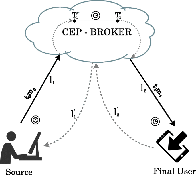
Overall schema of the stress test from a Source to Final User
-
CEP-Broker: it will be the entity that will analyse the information and generate the events turned into alarms. This entity will be the Local CEP and Broker located in the Fog Node (for the analysis of the fog computing architecture); or the Global CEP and Broker if you are in the Cloud (for cloud computing analysis).
-
Final User: will be the entity that will receive the alarms. For our study we have used a smartphone that will receive messages through the Internet, specifically through a 4G Connection.

Hence, tx refers to the topic to which the end-point is subscribed. mx is the message sent between the different entities, such that x=0 corresponds to the flow from Source to CEP-Broker, whereas x=1 corresponds to the flow from CEP-Broker to Final User. This message also includes its departure time. Note that we instrument the CEP-Broker to send back a message to the Source (and respectively, from the Final User to the CEP-Broker) to calculate an estimation of the one-way latency of the messages. We assume here that the upwards and backwards latency are the same.
Therefore, in this context the total time or latency (in seconds), Ltotal, from Source to Final User will be defined as the sum of times of several sectors, as shown in Equation 1.
Figure 6 details the procedure to calculate the times in each sector:
-
L1 will be the time since sending a message from Source to CEP-Broker, whose latency is denoted as l1, (Fog Node or Cloud). It should be noted that, for the calculation of this value, and due to the fact that the Broker has its own messaging manager making unfeasible to know exactly the time in which the alarm is distributed, a confirmation message, whose latency is represented as \(l^{\prime }_{1}\), will be sent. Notice that the shipment from Source will be made by subscription to the Broker. Therefore, the time spent sending the message t0m0 is defined according to Equation 2.
$$ L_{1} = \frac{l_{1} + l^{\prime}_{1}}{2} $$(2) -
LCEP will be the time in CEP, that is, the time in which the data reaches the CEP engine \(T^{\prime \prime }_{1}\), is analysed and the complex event in the form of an alarm, \(T^{\prime \prime }_{2}\) is obtained as output. Therefore, the analysis and generation time of the event is defined according to Equation 3.
$$ L_{{CEP}} = T^{\prime\prime}_{2} - T^{\prime\prime}_{1} $$(3) -
L2 will be the time since leaves the CEP engine, the alarm is published through the Broker and reaches the Final User, with a latency l2. Additionally, Final User will send a confirmation message, whose latency is \(l^{\prime }_{2}\). Thus, the latency in this last sector, when sending the t1m1 message, will be defined as shown in Equation 4.
$$ L_{2} = \frac{l_{2} + l^{\prime}_{2}}{2} $$(4)
To conclude this section, it should be noted that in the tests carried out on this model, whose results are shown in “Cloud vs. fog: latency evaluation with stress workload” section, the three entities (Source, CEP-Broker (Local and Global) and Final User) are located at different geographical points from the same city, and they have associated different public IP addresses. In addition, as mentioned, both for the data flow model in cloud computing and in fog computing represented in Fig. 5, the latency has been calculated with the same equations and following the same procedure.
Therefore, once the case study is defined, the data flow analysis and the latency study have been carried out, we will perform the performance evaluation for both architectures.
Fog & cloud computing: performance evaluation
This section begins with the description of the testbed where the evaluation tests have been carried out. Next, the CEP pattern that has been used in the tests, as well as the details of load generation will be specified. Already entering to the evaluation itself, a first analysis is presented on the impact of using various network technologies in the latency experienced by the end users of the system when receiving the generated events, depending on whether a fog or cloud computing architecture is used. Subsequently, a stress test is performed on both architectures taking into account the latency according to the number of alerts generated, to end with an analysis of the consumption of resources between both architectures.
Testbed description
Now the main hardware and software components of the testbed developed for carrying out the experiments will be described. The edge level of the testbed is deployed as a Python script that emulates 20 end-points and 2 gateways (10 end-points for each), namely, the Source entity in “Latency analysis” section. For the Fog Node, a Raspberry Pi 3 model B+ type microcomputer has been used, which has a 4-core 64-bit 1.4GHz processor, a 1GB RAM LPDDR2 SDRAM and Raspbian (without Graphical User Interface) operative system.
In order to keep control of the environment (i.e., network latencies), the core level has been implemented on-premise by using local resources. More precisely, the core level was implemented on an Intel Core i7 computer at 2.90GHzx8 with 8GB of RAM and 1TB of Hard Disk. Final User is a Huawei P20 Lite smartphone with Android version 8. A basic Android application has been developed in order to receive the alarms from CEP-Broker. As noted above, all the components have been deployed at different locations in Lima (Peru) and are interconnected through the public Internet.
The CEP engine used in this work is Apache Flink (version 1.8.0). Apache Flink is an open-source framework for state calculations on unlimited and limited data flows. Two types of processes are created during the runtime environment in Apache Flink. On the one hand, the Jobmanager implements 50 and 175 threads in Local and Global CEP, respectively, and is responsible for coordinating distributed execution, assignment of tasks, fault management, etc. On the other hand, the Taskmanager, configured with 512MB, is responsible for executing the tasks assigned by the Jobmanager on the data flow. The configuration of these two types of processes was optimised to minimize latency in the generation of alarms for our case study.
CEP pattern
The following is the implemented CEP pattern that will be used to analyse the incoming data, generate the events and notify with an alarm, in addition to the simulation of events that will be used to study the latency and performance set out in the next section.
In the tests performed, a CEP engine has been deployed for processing Closer-context events with a simple pattern. Thus, an alarm will be generated provided that, in moments of time t1 and t2, the values Vx(t1) and Vy(t2), received from different end-points, x and y, exceed a set threshold, Th. That is, it is true that Vx(t1)>Th & Vy(t2)>Th with t1<t2.
Thus, Fig. 7 shows an example of simulation until the second 120 to clarify the process of generating alarms. For our simulation a threshold Th=40 has been established. For the generation of events, it must be fulfilled that in consecutive moments a data arrives V1(t1) y V2(t2) such that V1(t1)>40 & V2(t2)>40 with t1<t2.

Simulation for the Generation of Events, Type Closer-Context Events, with CEP Pattern on a Time Line
The process is as follows (in that strict order):
-
1.
At the beginning, when it reaches CEP, the data V1(0)=40 is discarded for not fulfilling the condition.
-
2.
Upon arrival of the second data V2(40)=41 this is stored by fulfilling the first case of the employer.
-
3.
In the next 80 seconds another data arrives V3(80)=42 so the complete pattern has been fulfilled and, therefore, generates the event and we close this first case of alarm generation. Likewise, the first pattern is met again with this data, so we open a second case of event generation.
-
4.
In the second 120, we see that V4(120)=40 arrives so the pattern does not meet and the second case is discarded for not complying with the established rule.
It is important to note that the number of alarms can be increased by sending more topics in less timeframes, so we can set the maximum number of alarms per minute. Therefore, for all the tests, 10-minute simulations were made simulating a controlled number of alerts every minute in an equidistant manner, that is, 10 tests were carried out generating the same number of alerts every minute. For example, in a first round a consumption test was performed with the generation of 200 alarms per minute for 10 minutes; once the services are restarted, a load of 400 alarms is performed per minute for 10 minutes and the services are restarted.
For this work a maximum limit of 800 alarms/min has been established since when generating more alarms, a bottleneck was created in the Fog Node and events were beginning to be lost. To do this, 20 end-points are emulated and a total of 1600 data per minute is sent, that is, 80 data per end-point. Note that the load applied to the system is the same for all tests, varying only the number of alarms; therefore, the use of network bandwidth from Source is always the same.
Finally, it should be noted that for the following results, 30 tests were performed to ensure its accuracy. Mean values have been represented.
Influence of network technology on the latency
A key aspect of the proposed architecture is the network technology used by the Final Users (see Fig. 6). These elements can be connected to the Fog Node thanks to WAN networks or LAN networks depending on the location of the Final User. Performance depends on the technology used. Thus, in this section we are going to evaluate the impact of some of the most widely used technologies. More precisely, in these experiments we are going to evaluate the influence of 3 different technologies: 3G, 4G and WiFi on latency.
So, the testbed described in “Testbed description” section has been deployed considering 3 different Final Users, all of them subscribed to the Local Broker: (i) one is subscribed by WiFi (it is in its wireless LAN coverage area); and (ii) the other two are subscribed through 3G and 4G telephone networks respectively (WAN connection).
Hence, Fig. 8 shows the results of making this comparison between the different connections to the Broker for a load with the pattern described in the previous subsection and a total of 800 alarms/min. As expected, a user who is on the same LAN of the Fog Node (WiFi connection) will receive the alert in less time than one connected by 3G and 4G, although 4G is very close to WiFi. One of the strengths of 4G is the speed and stability of the signal with respect to 3G which, as can be seen, has a more pronounced variance than 4G [36].

Specification of the Latency Obtained in the Final User Entity for 3G, 4G and WiFi Connections
Thus, it can be seen from this study that the fog computing approach allows recipients in the area of coverage of the Fog Node to receive the alarm with a significantly lower latency than those recipients connected by telephony network. It should be noted that with a cloud computing approach, recipients can only receive the alert from the core level. The additional latencies incurred may be harmful for a wide range of applications.
Cloud vs. fog: latency evaluation with stress workload
Since the 4G telephony network has stable results and good latency performance, this will be the network used to send alarms to Final User in the remaining experiments. In addition, and as we will see in this section, this latency study should be extended so that we can compare if latency is reduced with the generation of Local Events (fog computing), rather than Global Events (cloud computing). Thus, in this particular case, and by which the subsequent performance study will be carried out, we will compare the latency in both architectures for a controlled number of alarms generated, specifically 200, 400, 600 and 800 alarms/min. Equation 1 has been used to calculate total latency (see “Latency analysis” section). In all the cases, averaged values for latencies are shown.
In this context, we can see in Fig. 9 how using a fog computing architecture reduces latency considerably, that is, the notification of an event arrives earlier to Final Users than in a cloud computing architecture.

Average Latency for the Different Loads Established, Comparing Fog Computing (FC) and Cloud Computing (CC)
Now, in this case we can see how the latency exceeds the second in the case of cloud computing. Moreover, it has a growing linear trend with a steep slope. On the other hand, fog computing also presents a linear trend, although it has much smoother slope, that is, it almost maintains a constant value. Therefore, we can consider that the latency in fog computing, in addition to being lower than in the cloud computing architecture, has a more stable value, independently of the assigned load.
In this context, the following test tries to determine which element of the architecture has the greatest impact on latency. For these results, the description of the latency and how to obtain it in each sector must be taken into account (see “Latency analysis” section). In particular, latencies in the three sectors are shown: (i) L1 time between the Source entity and before analysing in CEP (see Equation 2); (ii) TCEP time since a data is analysed and the event is generated (see Equation 3); and (iii) L2 time since the event becomes an alarm and reaches Final User (see Equation 4).
Therefore, Fig. 10 shows the average latency data, broken down by each sector indicated above. In it, it can be seen that in both architectures, the element that contributes most to latency is the MQTT Broker in the two phases of communication.

Average Latency Breakdown - Fog Computing (FC) vs. Cloud Computing (CC) Architectures
Taking into account the times obtained in the study of latency in Fig. 10 we can draw the following conclusions by sector:
-
L1 (see Fig. 10a): In this sector, the cloud computing architecture records a growing trend: the more alarms per minute there are, the higher latency L1. In the case of fog computing we can observe that the latency is constant and independent, as soon as we analyze a considerable set of events. Note that this parameter includes both the transmission time of the network and the work done by the MQTT Broker. In both architectures the communication latency has a low variance (see Fig. 8, 4G connection) so the variation observed in the latency values of the figure is due to the initialisation behaviour of the MQTT Broker as the first data arrives from Source.
-
TCEP (see Fig. 10b): The first behaviour to observe between both architectures is that the time observed in fog computing is slightly longer than the time in cloud computing because the resources in the Fog Node are more scarce than in the cloud. In any case, the time in both architectures is very similar and practically constant in this sector and, therefore, not very significant.
-
L2 (see Fig. 10c): For this sector we can see how, unlike L1, in both architectures there is a constant and independent trend to the number of alarms, because the Broker service is already initialised and it only distributes the alarms to the Final User. On the other hand, it is observed that in this case the latency for the cloud computing architecture is more than twice the one obtained by the fog computing architecture.
In summary, we can see that the growing trend in cloud computing (see Fig. 9) is due to the time spent in the L1 sector. In addition, an important factor that we can observe at this point has been that the MQTT Broker is a critical point of latency, while CEP performs the analysis of the data at a minimum latency.
Finally, not only latency is important to evaluate in both architectures. The distribution of computational resources in the different architectures must also be assessed.
Cost analysis: use of resources
In this section we will continue with the stress test developed for latency, but analysing the computational consumption for a fog computing architecture with respect to a cloud computing one. See Fig. 5 to remember the workflow in both architectures, analysing the distribution of resources at the core and edge level.
Case 1: core level
In the following results the measurements have been made in the core level, that is, in the central server (Cloud). The idea of this test is to know the computational consumption in the core level when using any of the architectures to evaluate. To this end, the Perf tool [37, 38] has been used to measure the energy consumed, Joules/millisecond (J/msec), and the Linux top tool to obtain the percentage of CPU and RAM consumed (see Fig. 11).

Performance Breakdown at the core level - Fog Computing (FC) vs. Cloud Computing (CC)
At first sight, we can see that cloud computing has a higher computational consumption in the measured values, so, by using a fog computing architecture we have reduced considerably the consumption of resources in the Cloud. The metrics evaluated are detailed below:
-
As for average CPU consumption (in %), see Fig. 11a, we can see that it has not been excessive in both architectures since the events sent do not perform complex mathematical operations that stress the CPU, but are simple comparison events. It can be seen that when cloud computing is used, CPU consumption is at most 1% higher than in fog computing, which is a very insignificant increase.
-
Regarding the consumption of RAM (in %), see Fig. 11b, we see more interesting results. It is possible to appreciate that the single activation of the CEP engine and the Broker represents a 35% increase in memory consumption. This aspect is due to the fact that CEP performs the analysis of events by storing data in the buffer and the Broker distributes the alarms from RAM. In contrast, in the case of fog computing, we see a very low value since the Broker and CEP services are not activated.
-
In matters of energy, see Fig. 11c, we see an average reduction of 69% in benefit of using fog computing with respect to cloud computing, without becoming high values. It is a consequence of the lower use of CPU and RAM.
It has been possible to verify how the use of fog computing download of work at the core level. This would be an additional benefit of the fog computing architectures (distribute resources across the different distributed devices) that will be more noticeable the more sophisticated the processing to be performed on the data.
Case 2: edge level
To obtain computational consumption at the edge level, when using a Raspberry Pi as Fog Node, only the consumption (in %) of CPU and RAM could be obtained because the Perf tool is not available for ARM processors. Therefore, the measurements made are now observed in Fig. 12. Note that the scales used in the graphs are different than in Case 1 (see Fig. 11). However, it is reported that the maximum energy consumption of a Raspberry Pi board at maximum load (i.e., the worst case) is 5.1W [39], leading to 0.0051J/msec, which is negligible compared to the energy consumed in the core level.

Performance Breakdown at the Edge Level - Fog Computing (FC) Vs. Cloud Computing (CC)
At first glance we can see how to use fog computing we have a greater consumption of resources in the Fog Node. This point is interesting and corroborates that the decrease in the consumption of computational resources in the core level implies a redistribution of resource usage towards the edge level. The metrics evaluated are detailed below:
-
Regarding the CPU consumption (in %), see Fig. 12a, we can observe for both architectures a linear behavior with the number of alarms processed per minute, although the slope obtained in the fog computing architecture is much steeper, reaching a consumption of 20% compared to 6% of cloud computing for 800 alarms/min. This is due to two facts: i) The limited performance of low-cost devices, such as the Raspberry Pi of our testbed; and ii) The workload since it is not only assigned by the CEP engine, but also that of the Broker who must make a double publication. However, the result obtained at this point is key: low-cost devices (less than US$40 per device) can be used to analyze data from IoT applications with real-time requirements using a CEP engine without overloading the system.
-
Regarding the consumption of RAM (in %), see Fig. 12b, it can be seen that the CEP and Broker engine consume up to 80% of the RAM in the Fog Node, that is, almost 70% more than in the cloud computing model, since in the latter case the Fog Node is a passive element. Like the core level analysis, CEP performs the event analysis and the Broker distributes the alarms from RAM. A key aspect that certifies the feasibility of using low-cost devices is that the % of memory in use is constant and independent of the number of alarms generated.
As a summary, we can observe that the assignment of tasks and work to the edge level with CEP and Broker brings with them a distribution of work assigned to the Fog Nodes while the core level has a much lower load. This is an interesting fact since in addition to harnessing the computing power at the edge level, it also highlights that the response times to the end user are much shorter, which in turn enables the deployment of a large number of applications with real-time requirements in IoT.
Conclusions and future plans
This paper shows the development of a distributed fog computing architecture for the deployment of IoT applications. Our study shows how these architectures optimise the distribution of resources throughout the entire deployed platform, in addition to considerably reducing latency.
On the one hand, regarding resource distribution, we have observed that by deploying critical data analysis and decision-making applications (CEP and the MQTT Broker, in our case), the values of the evaluated metrics are reduced considerably (CPU consumption, RAM memory and power consumption) on the cloud server, with the consequent savings for the cloud provider. Specifically, the fog computing approach enables a reduction of RAM consumption up to 35% and energy up to 69% at the core level, since it fully exploits the computational resources of fog nodes. In addition, it has been verified that low-cost devices, such as Raspberry Pi with a cost less than US$40, have enough computing resources to offer the quality of service required by IoT applications with real-time needs.
On the other hand, regarding latency, the work highlights how a fog computing architecture considerably reduces latency with respect to cloud computing, up to 35% better. Breaking down the latency results, we can also see how the Broker is the critical element of the increase in latency.
Regarding future work, the authors of this work consider it appropriate to evaluate Software Defined Networks (SDN) techniques in the Fog Nodes. As observed in the document, the limit of 800 alarms/min can be mitigated by developing a spine-leaf layer between the core and edge level, which allows the analysis to be redirected in case of Fog Node overload.
Likewise, a study on the creation of micro services in the Fog Node for the Broker and CEP through containers would be very interesting to provide a certain degree of isolation between different applications deployed on the edge level. To do this, using microclouds techniques in the Fog Node can be an interesting aspect for reducing consumption and latency.
Finally, it is proposed to use more sophisticated microcomputers that have built-in accelerators (graphics cards, Tensor Processing Units (TPUs), …) to analyse the impact of deriving machine and deep learning techniques from the Cloud to the Fog Node.
Availability of data and materials
The analysis code is available in JAVA language program for the CEP analysis (.java files).
Notes
The identification and generation of a complex event will be also referred to as an alarm throughout this paper.
References
Omale G (2018) Gartner Identifies Top 10 Strategic IoT Technologies and Trends. https://www.gartner.com/en/newsroom/press-releases/2018-11-07-gartner-identifies-top-10-strategic-iot-technologies-and-trends. Accessed 21 Dec 2020.
Yannuzzi M, van Lingen F, Jain A, Parellada OL, Flores MM, Carrera D, Pérez JL, Montero D, Chacin P, Corsaro A, et al. (2017) A new era for cities with fog computing. IEEE Internet Comput 21(2):54–67.
Sarkar S, Chatterjee S, Misra S (2018) Assessment of the Suitability of Fog Computing in the Context of Internet of Things. IEEE Trans Cloud Comput 6(1):46–59. https://doi.org/10.1109/TCC.2015.2485206.
Mahmud R, Koch FL, Buyya R (2018) Cloud-fog interoperability in IoT-enabled healthcare solutions In: Proceedings of the 19th International Conference on Distributed Computing and Networking, 32.. ACM, Varanasi.
Xiong Z, Feng S, Wang W, Niyato D, Wang P, Han Z (2018) Cloud/fog computing resource management and pricing for blockchain networks. IEEE Internet Things J 6(3):4585–4600.
Luan TH, Gao L, Li Z, Xiang Y, Wei G, Sun L (2015) Fog computing: Focusing on mobile users at the edge. ArXiv:1502.01815. https://arxiv.org/abs/1502.01815.
Roman R, Lopez J, Mambo M (2018) Mobile edge computing, fog et al.: A survey and analysis of security threats and challenges. Futur Gener Comput Syst 78:680–698.
Rahmani AM, Liljeberg P, Preden J-S, Jantsch A (2017) Fog computing in the internet of things: Intelligence at the edge, 17–31.. Springer International Publishing. https://doi.org/10.1007/978-3-319-57639-8.
Barik RK, Dubey H, Misra C, Borthakur D, Constant N, Sasane SA, Lenka RK, Mishra BSP, Das H, Mankodiya K (2018) Fog assisted cloud computing in era of big data and internet-of-things: systems, architectures, and applications In: Cloud Computing for Optimization: Foundations, Applications, and Challenges. Studies in Big Data, vol 39, 367–394.. Springer, Cham. https://doi.org/10.1007/978-3-319-73676-1_14.
Dignan LWhat’s next for data centers? Think micro data centers. https://www.zdnet.com/article/whats-next-for-data-centers-think-micro-data-centers/. Accessed 21 Dec 2020.
Xu Z, Zhang Y, Li H, Yang W, Qi Q (2020) Dynamic resource provisioning for cyber-physical systems in cloud-fog-edge computing. J Cloud Comput 9(1):1–16.
Devnet CWhat is IOx?https://developer.cisco.com/docs/iox/. Accessed 21 Dec 2020.
Bonomi F, Milito R, Zhu J, Addepalli S (2012) Fog computing and its role in the internet of things In: Proceedings of the first edition of the MCC workshop on Mobile cloud computing, 13–16.. ACM, Helsinki.
Wu C, Li W, Wang L, Zomaya A (2018) Hybrid Evolutionary Scheduling for Energy-efficient Fog-enhanced Internet of Things. IEEE Trans Cloud Comput:1–1. https://doi.org/10.1109/TCC.2018.2889482.
Garcia-de-Prado A, Ortiz G, Boubeta-Puig J (2017) COLLECT: COLLaborativE ConText-aware service oriented architecture for intelligent decision-making in the Internet of Things. Expert Syst Appl 85:231–248.
Goudarzi M, Wu H, Palaniswami MS, Buyya R (2020) An Application Placement Technique for Concurrent IoT Applications in Edge and Fog Computing Environments. IEEE Trans Mob Comput 20(4):1–1.
Mahmud R, Ramamohanarao K, Buyya R (2020) Application Management in Fog Computing Environments: A Taxonomy, Review and Future Directions. ACM Comput Surv 53(4). https://doi.org/10.1145/3403955.
Yousefpour A, Fung C, Nguyen T, Kadiyala K, Jalali F, Niakanlahiji A, Kong J, Jue JP (2019) All one needs to know about fog computing and related edge computing paradigms: A complete survey. J Syst Archit 98:289–330. https://doi.org/10.1016/j.sysarc.2019.02.009.
Dolui K, Datta SK (2017) Comparison of edge computing implementations: Fog computing, cloudlet and mobile edge computing In: 2017 Global Internet of Things Summit (GIoTS), 1–6. https://doi.org/10.1109/GIOTS.2017.8016213.
Dastjerdi AV, Gupta H, Calheiros RN, Ghosh SK, Buyya R (2016) Chapter 4 - fog computing: principles, architectures, and applications. In: Buyya R Vahid Dastjerdi A (eds)Internet of Things, 61–75.. Morgan Kaufmann. https://doi.org/10.1016/B978-0-12-805395-9.00004-6.
Yick J, Mukherjee B, Ghosal D (2008) Wireless sensor network survey. Comput Netw 52(12):2292–2330. https://doi.org/10.1016/j.comnet.2008.04.002.
Bellavista P, Berrocal J, Corradi A, Das SK, Foschini L, Zanni A (2019) A survey on fog computing for the Internet of Things. Pervasive Mob Comput 52:71–99.
Haghi Kashani M, Rahmani AM, Jafari Navimipour N (2020) Quality of service-aware approaches in fog computing. Int J Commun Syst 33(8):4340. https://doi.org/10.1002/dac.4340.
Naik N (2017) Choice of effective messaging protocols for IoT systems: MQTT, CoAP, AMQP and HTTP In: 2017 IEEE International Systems Engineering Symposium (ISSE), 1–7.. IEEE, Vienna.
MQTT.org (2021) MQTT: The Standard for IoT Messaging. https://mqtt.org/. Accessed 4 Mar 2021.
Luckham DC (2011) Event Processing for Business: Organizing the Real-time Enterprise. Wiley.
Nasiri H, Nasehi S, Goudarzi M (2019) Evaluation of distributed stream processing frameworks for IoT applications in Smart Cities. J Big Data 6(52). https://doi.org/10.1186/s40537-019-0215-2.
Dhillon AS, Majumdar S, St-Hilaire M, El-Haraki A (2018) Mcep: A mobile device based complex event processing system for remote healthcare. IEEE Int Conf Internet Things: 203–210. https://doi.org/10.1109/Cybermatics_2018.2018.00064.
Fernández-Caramés TM, Fraga-Lamas P, Suárez-Albela M, Díaz-Bouza MA (2018) A fog computing based cyber-physical system for the automation of pipe-related tasks in the industry 4.0 shipyard. Sensors 18(6). https://doi.org/10.3390/s18061961.
Varghese B, Wang N, Nikolopoulos DS, Buyya R (2017) Feasibility of fog computing. ArXiv: 1701.05451. https://arxiv.org/abs/1701.05451.
Castillo-Cara M, Huaranga-Junco E, Quispe-Montesinos M, Orozco-Barbosa L, Antúnez EA (2018) FROG: a robust and green wireless sensor node for fog computing platforms. J Sensors 2018:1–12.
Okafor KC, Achumba IE, Chukwudebe GA, Ononiwu GC (2017) Leveraging fog computing for scalable IoT datacenter using spine-leaf network topology. J Electr Comput Eng 5(4):3246–3257.
Shah-Mansouri H, Wong VWS (2018) Hierarchical Fog-Cloud Computing for IoT Systems: A Computation Offloading Game. IEEE Internet Things J 5(4):3246–3257.
Jalali F, Hinton K, Ayre R, Alpcan T, Tucker RS (2016) Fog computing may help to save energy in cloud computing. IEEE J Sel Areas Commun 34(5):1728–1739.
Morabito R (2017) Virtualization on Internet of Things edge devices with container technologies: a performance evaluation. IEEE Access 5:8835–8850.
Shi C, Ren Z, Yang K, Chen C, Zhang H, Xiao Y, Hou X (2018) Ultra-low latency cloud-fog computing for industrial internet of things In: 2018 IEEE Wireless Communications and Networking Conference (WCNC), 1558–2612.. IEEE, Barcelona.
perf (2019) perf: Linux profiling with performance counters. https://en.wikipedia.org/wiki/Perf_(Linux). Accessed 21 Dec 2020.
Lovón-Melgarejo J, Castillo-Cara M, Huarcaya-Canal O, Orozco-Barbosa L, García-Varea I (2019) Comparative Study of Supervised Learning and Metaheuristic Algorithms for the Development of Bluetooth-Based Indoor Localization Mechanisms. IEEE Access 7:26123–26135.
Geerling J (2020) Power Consumption Benchmarks. https://www.pidramble.com/wiki/benchmarks/power-consumption. Accessed 21 Dec 2020.
Acknowledgements
Not applicable
Funding
This work has been partially funded by the Spanish Ministry of Science, Innovation and Universities (ref. RTI2018-098156-B-C52), by the Research Plan of the University of Castilla-La Mancha (ref. 2019-GRIN-27060), and by FONDECYT / World Bank (ref. 026-2019 FONDECYT-BM-INC.INV).
Author information
Authors and Affiliations
Contributions
Authors’ contributions
G. Mondragón-Ruiz and A. Tenorio-Trigoso has directed the Conceptualisation, Data Curation, Formal Analysis, Writing – Original Draft Preparation, Writing – Review & Editing. M. Castillo-Cara, M. B. Caminero and C. Carrión have directed the Conceptualisation, Formal Analysis, Writing – Review & Editing. All authors reviewed and approved the final manuscript.
Authors’ information
Giovanny Mondragón-Ruiz, received the B.Sc. degree in Computer Science from the Universidad Nacional de Ingenieria (UNI) from Lima - Perú in 2018. He is currently a member of Intelligent Ubiquitous Technologies – Smart City (IUT-SCi) Lab at the Universidad Nacional de Ingeniería. He is researching Edge Level Architectures and Fog Computing optimizations. His research interests include Complex Event Processing, Mobile Computing and Internet of Things.
Alonso Tenorio-Trigoso received the M.Sc. degree and he is studying the PhD in Computer Science from the UCLM, Albacete, Spain. He has been working on university educational issues at the Computer Science as an Associate Professor and a member of IUT-SCi Lab at UNI. His research interests includes Distributed Computing, IoT technologies and Internet protocols.
Manuel Castillo-Cara received the PhD degree from the University of Castilla-La Mancha (UCLM) in July 2018. He has been working on university educational issues at the Computer Science as an Associate Professor and head of Intelligent Ubiquitous Technologies – Smart City (IUT-SCi) Lab at Universidad de Lima. His current research is focused on Intelligent Ubiquitous Technologies, especially on in Wireless Sensor Networks, Distributed Computing, Pattern Recognition and Artificial Intelligence.
Blanca Caminero is an Associate Professor in Computer Architecture and Technology at the Computing Systems Department at UCLM. She teaches networking related subjects at the School of Computer Science and Engineering in Albacete since 2000. She holds a Ph.D. Degree in Computer Science from the UCLM, and her current research interests are QoS support and efficient resource scheduling in distributed systems (Cloud, Fog, Edge…). She is a member of the IEEE.
Carmen Carrión is an Associate Professor in Computer Architecture and Technology at the Computing Systems Department at the UCLM. She holds a Ph.D. Degree in Physics from the University of Cantabria, and her interests include resource management schemes, virtualization technologies and QoS in Fog-IoT frameworks.
Corresponding author
Ethics declarations
Competing interests
The authors declare that they have no competing interests.
Additional information
Publisher’s Note
Springer Nature remains neutral with regard to jurisdictional claims in published maps and institutional affiliations.
Rights and permissions
Open Access This article is licensed under a Creative Commons Attribution 4.0 International License, which permits use, sharing, adaptation, distribution and reproduction in any medium or format, as long as you give appropriate credit to the original author(s) and the source, provide a link to the Creative Commons licence, and indicate if changes were made. The images or other third party material in this article are included in the article’s Creative Commons licence, unless indicated otherwise in a credit line to the material. If material is not included in the article’s Creative Commons licence and your intended use is not permitted by statutory regulation or exceeds the permitted use, you will need to obtain permission directly from the copyright holder. To view a copy of this licence, visit http://creativecommons.org/licenses/by/4.0/.
About this article

Cite this article
Mondragón-Ruiz, G., Tenorio-Trigoso, A., Castillo-Cara, M. et al. An experimental study of fog and cloud computing in CEP-based Real-Time IoT applications. J Cloud Comp 10, 32 (2021). https://doi.org/10.1186/s13677-021-00245-7
Received:
Accepted:
Published:
DOI: https://doi.org/10.1186/s13677-021-00245-7