Fast methods for designing circulant network topology with high connectivity and survivability

Rui Lu

doi:10.1186/s13677-016-0056-x

Research
Open Access

Fast methods for designing circulant network topology with high connectivity and survivability

Rui Lu¹Email author

Journal of Cloud ComputingAdvances, Systems and Applications20165:5

https://doi.org/10.1186/s13677-016-0056-x

Received: 8 January 2016
Accepted: 18 April 2016
Published: 5 May 2016

Abstract

This paper proposes two fast methods to design network topologies with high connectivity and survivability based on circulant graph theory. The first method, namely, the Combination Method (CM), investigates the average distances of circulant graphs with different combinations of chordal jumps, and tries to locate the optimal one among them. For this purpose, empirical formulas are proposed to describe the fluctuation features of average distances on curved surfaces. Furthermore, an enhanced Local Search Method (LSM) is proposed to find the local minimum points in troughs of the surfaces. The second method, namely, the Spider Web Method (SWM), is based on a bionic concept deriving from observation of the spider web, which is a classical example of network connectivity and survivability in natural world. The relation between CM and SWM in certain situations is also discussed. Finally, the connectivity and survivability of the topologies designed by CM and SWM are verified via simulated experiments involving vertex destruction.

Keywords

Network
Topology design
Circulant graph
Average distance
Local search method

Introduction

Topology design plays an important role in network planning. Various topologies have been studied and analyzed for different networks [1–3]. A circulant graph outperforms other topologies owing to its low message delay, high connectivity, and strong survivability [4–8]. Therefore, it has been widely employed in many technical fields such as telecommunication networks, computer networks, parallel processing systems, and social networks [9–12].

The connectivity and survivability of circulant graph networks can be evaluated by several metrics, such as average distance and connectivity ratio [2, 12–15]. The average distance is preferred as the prime optimization objective for it effectively represents network connectivity. In general, the smaller the average distance is, the shorter the delay is. Although network with complete graph topology has the minimum average distance of 1, the demand of a huge number of nodes and link resources usually render it impractical in projects. Therefore, the performance of circulant graphs with limited resources is a major focus of network planning. Lower bounds and heuristic algorithms locating the minimum average distance of a circulant graph have been proposed [2, 6, 15]. Furthermore, the average distance of a recursive circulant graph, i.e., a special type of circulant graph, has also been investigated [16]. However, the optimal jump sequence of a circulant graph can be determined only when its degree is 4.

In this paper, we propose two fast methods to construct network topology with small average distance and high connectivity ratio based on circulant graph theory and bionics. Furthermore, we verify the effectiveness of the proposed methods by simulated experiments.

The remainder of this paper is organized as follows: In section Definitions of chordal ring, average distance and connectivity ratio, the concepts of circulant graphs and evaluation metrics are introduced. In section The Combination Method for topology design, we propose a Combination Method (CM) that develops formulas and algorithms to construct a circulant graph with a relatively minimum average distance, based on the features and characteristics of the average distance fluctuation curves. A Local Search Method (LSM) is also developed to optimize the search for the jump sequence with the minimum average distance. In section The Spider Web Method for topology design, we propose a more intuitive design method, namely, the Spider Web Method (SWM). This method is typically effective when the degree of each node is 4. In section Survivability experiments, survivavility experiments are implemented to verify the survivability of topologies designed by CM and SWM. Different nodes and links are destroyed enumerately, and the worst connectivity ratios of the networks are recorded and compared. Finally, research results in this paper are summarized and concluded.

Definitions of chordal ring, average distance and connectivity ratio

Circulant graph and chordal ring

A circulant graph is a special case of a Cayley graph. Suppose that G(V, E) (V = {v ₁, v ₂, …,v _m}, E = {e ₁, e ₂, …, e _n}) is a graph with m vertices and n edges. The circulant graph can be defined as follows [2, 13]:

Definition 1: G(V, E) is a simple graph with m vertices and n edges. There are integers w ₁, w ₂, …, w _j (w ₁ < w ₂ < … < w _j < (m + 1)/2) that represent a jump sequence. Two vertices v_k and v_l of V are connected if and only if (k + w _i) mod m = l, or (k – w _i) mod m = l. This graph is defined as a circulant graph. A circulant graph with j jumps is usually denoted by CG(m; w ₁, w ₂, …, w _j) or CG(m; W) with jump sequence W = {w ₁, w ₂, …, w _j}, and |W| = j.
This definition does not guarantee that a circulant graph is connected. For example, CG(8; 1, 2) is a connected circulant graph, but CG(8; 2, 4) is not connected. Boesch and Tindell [5] found that a circulant graph is connected if and only if the greatest common divisor gcd(m, w ₁, w ₂, …,w _j) is equal to 1. Such a graph is always known as a connected circulant graph. Furthermore, it has been proved that every connected circulant graph has a Hamiltonian cycle [17]. In particular, a complete graph can always be considered as a combination of all CG(m; w _i) (1 ≤ i ≤ ⌊m/2⌋), which are considered as basic parts, as shown in Fig. 1.

Fig. 1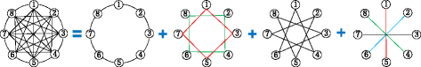
Decomposition of a complete graph
In addition, the chordal ring network is introduced. There are two definitions for a chordal ring [13].
Definition 2: If a circulant graph CG(m, W) has w ₁ equal to 1, it is known as a chordal ring. The edges with w _i ≠ w ₁ (2 ≤ i ≤ j) are denoted by chords of length w _i.
Definition 3: G(V, E) is a simple graph with m vertices and n edges. Vertices v ₁, v ₂, …,v _m in V are connected in sequence into a Hamiltonian cycle. There are integers w ₁, w ₂, …, w _j (w ₁ < w ₂ < … < w _j < (m + 1)/2). Two vertices v _k and v _l of V are connected if and only if k and l are odd numbers, and (k + w _i) mod m = l. This graph is defined as a chordal ring. A circulant graph with j chords is usually denoted by CR(m, w ₁, w ₂, …, w _j) or CR(m, W).
In this work, we consider the former definition of a chordal ring, i.e., Definition 2. From this definition, it can be deduced that a chordal ring is a special case of a connected circulant graph.

Average distance

The average distance $ \overline{D} $ is defined as the average length of the shortest paths between any two nodes in the network [2]. It is illustrated on the basis of bi-directed graphs, which are essentially undirected graphs with edges represented by bi-directed arrows instead of full lines [18]. $ \overline{D} $ can be expressed as

$$ \overline{D}=\frac{{\displaystyle {\sum}_{v_i\in V}{\displaystyle {\sum}_{v_j\in V,{v}_j\ne {v}_i}{D}_{ij}}}}{m\left(m-1\right)} $$

(1)

D _ij is the shortest path distance between vertices v _i and v _j. In general, the shortest path distance can be expressed as

$$ {D}_{ij}= \min {\displaystyle {\sum}_{e_{ij}\in E}{c}_{ij}{x}_{ij}} $$

$$ s.t.\kern1em {\displaystyle {\sum}_{j:{e}_{ij}\in E}{x}_{ij}}-{\displaystyle {\sum}_{j:{e}_{ji}\in E}{x}_{ji}}=\kern0.5em \left\{\begin{array}{c}\hfill \kern0.5em 1,\hfill \\ {}\hfill -1,\hfill \\ {}\hfill \kern0.74em 0,\hfill \end{array}\right.\kern0.5em \begin{array}{c}\hfill i=s,\hfill \\ {}\hfill i=t,\hfill \\ {}\hfill \kern0.36em i\ne s,t.\hfill \end{array}\kern1em {x}_{ij}\ge 0 $$

(2)

In the definition of D _ij, x _ij denotes whether there is an edge e _ij from v _i to v _j on the path from v _s to v _t, and c _ij denotes the cost of edge e _ij. They can be expressed as follows:

$$ {x}_{ij}=\left\{\begin{array}{c}\hfill 1\hfill \\ {}\hfill 0\hfill \end{array}\right.\kern2em \begin{array}{c}\hfill {e}_{ij}\; is\; on\; the\; path\; from\;{v}_s\;to\;{v}_t\kern0.84em \hfill \\ {}\hfill {e}_{ij}\; is\; not\; on\; the\; path\; from\;{v}_s\;to\;{v}_t\hfill \end{array} $$

(3)

$$ {c}_{ij}=\left\{\begin{array}{c}\hfill 1\kern0.48em \hfill \\ {}\hfill +\infty \hfill \end{array}\right.\kern1em \begin{array}{c}\hfill If\; there\; is\; an\; edge\; between\;{v}_i\; an d\;{v}_j\hfill \\ {}\hfill If\; there\; is\; no\; edge\; between\;{v}_i\; an d\;{v}_j\hfill \end{array} $$

(4)

According to the isomorphism of a circulant graph, $ \overline{D} $ can be simplified as [19–23]

$$ \overline{D}=\frac{{\displaystyle {\sum}_{v_j\in V,{v}_j\ne {v}_1}{D}_{1j}}}{m-1} $$

(5)

A typical lower bound for the average distance is the Moore bound [2]. However, the Moore bound is attainable only for some special topologies [2, 6].

A circulant graph with a jump relatively prime with m is isomorphic to a chordal ring. Therefore, its average distance is equal to that of the corresponding chordal ring. In most cases, the optimal distance of a chordal ring is equal to that of a circulant with the same m. The smallest m that does not fit this rule is 450, according to the exhaustive research of Fiol [24, 25].

According to the definition of a circulant graph, there are C(⌊m/2⌋ , j) circulant graphs with different W for certain m and j. Correspondingly, the number of chordal rings for the same m and j is C(⌊m/2⌋ − 1, j − 1), which is j/⌊m/2⌋ the number of circulants on the same scale.

Connectivity ratio

Connectivity ratio is defined as the ratio of the number of reachable node pairs to the total number of node pairs in the network, and it can be calculated as$ C=\frac{{\displaystyle {\sum}_{i\in V}{\displaystyle {\sum}_{j\in V,j\ne i}{l}_{ij}}}}{m\left(m-1\right)}, $ subject to

$$ {l}_{ij}=\left\{\begin{array}{c}\hfill 1\kern1em there\kern0.5em is\kern0.5em a\kern0.5em path\kern0.5em from\kern0.5em {v}_i\kern0.5em to\kern0.5em {v}_j\kern0.1em ;\kern0.6em \hfill \\ {}\hfill 0\kern1em there\kern0.5em is\kern0.5em no\kern0.5em path\kern0.5em from\kern0.5em {v}_i\kern0.5em to\kern0.5em {v}_j\kern0.1em .\hfill \end{array}\right. $$

(6)

The maximum network connectivity ratio for a network with q node failures can be expressed as

$$ {C}_{q, \max }=\frac{\left(m-q\right)\left(m-q-1\right)}{m\left(m-1\right)} $$

(7)

Assuming that the probability of q node failures is p _q, we propose the probability weighted connectivity, calculated as $ \overline{C}={\displaystyle {\sum}_{q=1}^m{p}_q{C}_q} $

$ \overline{C} $ is more suitable for measuring network survivability in the event of a disaster that may take a heavy toll.

The Combination Method for topology design

Average distance of chordal ring

In this section, the average distance of a chordal ring is calculated in an enumerated manner, and some characteristics are deduced. The number of edges in a chordal ring CR(m, W) is given by

$$ n=\left\{\begin{array}{c}\hfill jm\begin{array}{cc}\hfill \hfill & \hfill \begin{array}{cc}\hfill \begin{array}{cc}\hfill \hfill & \hfill \hfill \end{array}\hfill & \hfill {w}_j\ne \frac{m}{2}\hfill \end{array}\hfill \end{array}\hfill \\ {}\hfill \left(j-\frac{1}{2}\right)m\begin{array}{cc}\hfill \hfill & \hfill \kern0.32em {w}_j=\frac{m}{2}\hfill \end{array}\hfill \end{array}\right.\kern2em \begin{array}{c}\hfill \hfill \\ {}\hfill \left(1\le j\le \frac{m}{2}\right)\hfill \\ {}\hfill \hfill \end{array} $$

(8)

The average distance of chordal rings for j = 1 and 2 has already been investigated; however, the average distance of more general chordal rings is still being studied. All these chordal rings are discussed stepwise:

①
If j = 1, n is equal to m (m ≥ 3) and the chordal ring is a Hamiltonian cycle. The average distance of the Hamiltonian cycle can be deduced from the following proposition:
- Proposition 1: G(V, E) is a Hamiltonian cycle, |V| = m (m ≥ 3), |E| = n (n = m). If m is odd, its average distance is (m + 1)/4; if m is even, its average distance is (1/4)[1/(m − 1) + m + 1].
②

If j = 2, the average distance of the chordal rings can be expressed as a function $ \overline{D}=f\left(m,{w}_1,{w}_2\right) $ with w ₁ = 1. However, this function becomes too complex to be expressed analytically. We draw a curve that connects discrete average distance points that vary with w ₂, as shown in Fig. 2. This figure shows 3 features of the average distance that varies with w ₂-jump:

Fig. 2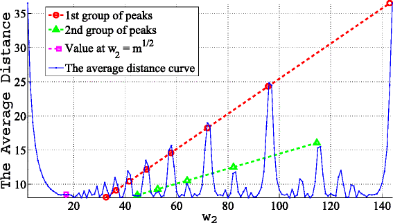
Increasing tendency of peak values for average distance of chordal ring with m = 289 and j = 2

First, there are several local minimum values scattered in the troughs among several local peak values. The values of the local minimum average distances do not differ significantly and are very close to the values of the global minimum points among them. All of them contribute to the flat envelope at the bottom of the curve.

Second, there are local maximum average distance points near (2/k)w _max, [4/(2k + 1)]w _max (k ≥ 2), where w _max = ⌊m/2⌋. The values of the peaks are approximately linearly proportional to their positions when k is small. Specifically, the average distance is nearly $ \left(2/k\right){\overline{D}}_{\max } $ at points w ₂ = (2/k)w _max. Further, $ {\overline{D}}_{\max } $ is the average distance when w ₂ = w _max. However, if k is large, the peaks cannot be resolved and is no longer linearly proportional to its position. The peaks can clearly be observed along the red and green lines in Fig. 2.

The tendency of the optimal average distances varying with m is presented in Fig. 3. Although it has been proved that the average distance does not increase monotonically with m [24], it approximately has a relation with m. From Fig. 3, the global minimum average distance in our topology with n = 2 m is nearly proportional to $ \sqrt[2]{m} $. The relation between $ {\overline{D}}_{\min } $ and m can be represented approximately as
$$ {\overline{D}}_{\min}\approx 0.47\left(\sqrt[2]{m}-\sqrt[2]{5}\right)+1 $$

(9)

Fig. 3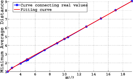
Global optimal average distance varying with $ \sqrt[2]{m} $
③

If 2 < j ≤ ⌊m/2⌋, the average distance of the chordal ring can be expressed as a function as follows:
$$ \begin{array}{c}\hfill \hfill \\ {}\hfill \overline{D}=f\left(m,{w}_1,\dots \kern0.2em ,{w}_i,\dots \kern0.2em ,{w}_j\right)\kern1.1em \hfill \\ {}\hfill \hfill \end{array}\left(\begin{array}{c}\hfill {w}_1=1\hfill \\ {}\hfill 2<{w}_i\le \left\lfloor \frac{m}{2}\right\rfloor, 2\le i\le j\hfill \\ {}\hfill {w}_i<{w}_k,i<k\le j\hfill \end{array}\right) $$

(10)

There are C(⌊m/2⌋ − 1, j − 1) choices for W = {w ₁, w ₂, …,w _j}. Figure 4 shows an example of $ \overline{D} $ varying with w ₂ and w ₃ (w ₁ = 1). Even though the curved surface is rough, the envelope of the local minimum points is on a relatively flat surface. In Fig. 11, several peak sequences can be found radiating with increasing peak values from positions where w ₂ and w ₃ are small. They are local maximum points at (w ₂, w ₃), with w ₃ near (2/k)w _max or [4/(2k + 1)]w _max and w ₂ near (2/s)w ₃ or [4/(2s + 1)]w ₃ (k ≥ 2, s ≥ 2).

Fig. 4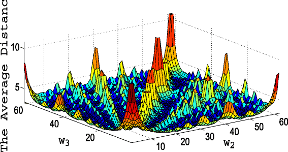
Average distance with m = 125 and j = 3

Empirical formulas of the minimum average distance values are also studied by a curve fitting method. The shortest average distance varying with j and m can be approximately expressed as
$$ {\overline{D}}_{\min}\left(j,m\right)\approx \left\{\begin{array}{c}\hfill \begin{array}{cc}\hfill \frac{j}{4}\left[0.94+\frac{4j-5}{m}\right]\kern0.22em \left[{m}^{\frac{1}{j}}-{\left(2j+1\right)}^{\frac{1}{j}}\right]+1\hfill & \hfill 2\le j<\left\lfloor \frac{m}{2}\right\rfloor \hfill \end{array}\hfill \\ {}1\begin{array}{cc}\hfill \hfill & \hfill \hfill \end{array}\begin{array}{cc}\hfill \hfill & \hfill \hfill \end{array}\begin{array}{cc}\hfill \hfill & \hfill \hfill \end{array}\begin{array}{cc}\hfill \hfill & \hfill \hfill \end{array}\begin{array}{cc}\hfill \hfill & \hfill \hfill \end{array}\begin{array}{cc}\hfill \hfill & \hfill \hfill \end{array}\begin{array}{cc}\hfill \hfill & \hfill \hfill \end{array}\begin{array}{cc}\hfill \begin{array}{cc}\hfill \hfill & \hfill \hfill \end{array}\hfill & \hfill j\ge \left\lfloor \frac{m}{2}\right\rfloor \hfill \end{array}\hfill \end{array}\right. $$

(11)

To verify the effectiveness of the formula, we compare the real $ {\overline{D}}_{\min } $ selected in enumerated manner according to the definition of average distance, with that calculated using formula (11). The result is presented in Fig. 5. According to the empirical formula described above, $ {\overline{D}}_{\min } $ is approximately proportional to j m ^1/j.

Fig. 5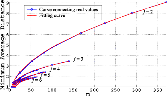
Variation of global optimal average distance with m for different j

The Combination Method

The idea of Combination Method is to select the optimal combination of chordal jumps by avoiding the peaks on the curved surface of the average distance. The formula for different number of jumps (j) is proposed as follows.

①

If j = 2, the average distance curve has a rough surface which does not vary monotonous with w ₂ and is hard for choosing the optimal w ₂-jump. However, if the peak positions can be avoided, some local minimum points are still locatable. In this work, two peak avoidance methods are developed:

The first method is Global Peak Avoidance (GPA). As shown by the pink marker in Fig. 6, there is a relatively slow varying region that has very small average distance values. Although the values may not be the global minimum points, they are very close to the optimal ones. We can quantitatively locate w ₂-jump in this region as
$$ {w}_2=\left\lfloor \sqrt[2]{m}\right\rfloor $$

(12)

Fig. 6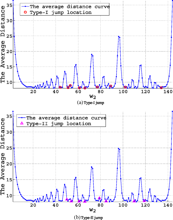
The jumps chosen by CM. a Type-I jump. b Type-II jump

For example, for m = 289, w ₂ = 17, and the corresponding $ {\overline{D}}_{sel} = 8.5 $. This is very close to the minimum average distance of 8.0278.

The second method is Local Peak Avoidance (LPA). This method derives from the motivation to select jump sequence W in the trough between peaks near the positions of (2/k)w _max, [4/(2k + 1)]w _max.
$$ {w}_2=\left\lfloor \left(2/k\right){w}_{\max}\pm \beta \right\rfloor, \kern1em \beta =\sqrt[2]{\left[\frac{2}{k}-\frac{2}{k+1}\right]m} $$

(13)

$$ {w}_2=\left\lfloor \left[4/\left(2k+1\right)\right]{w}_{\max}\pm \gamma \right\rfloor, \kern1em \gamma =\sqrt[2]{\left[\frac{4}{2k+1}-\frac{2}{k+1}\right]\left(\frac{m}{2}\right)} $$

(14)

The former w ₂ is termed as Type-I jump, whereas the latter is termed as Type-II jump.

A simulation is implemented to verify these formulas. The chordal ring with m = 289 is still considered as an instance. For Type-I jump, select k = {2, 3, 4, 5, 6}, and calculate w ₂ that complies with the Type-I jump formula (13). After the removal of w ₂ from the range of (1, w _max), the results are obtained as shown in Fig. 6 (a). Similarly, for the Type-II jump, select k = {2, 3, 4, 5}, and calculate w ₂ that complies with the Type-II jump formula (14). The results are shown in Fig. 6 (b). The mean value of the average distance of the Type-I jump location $ {\overline{D}}_{sel- Type-I} $ is 8.3927, and that of the Type-II jump location $ {\overline{D}}_{sel- Type-II} $ is 8.3733. They are also very close to the optimal average distance of 8.0278.

②

If j = 3, troughs with relatively small values on the average distance surface can also be found. Similarly, this can be accomplished by avoiding local peaks. We select two types of W = (1, w ₂, …, w _i, …, w _j) (2 ≤ i < j). For the Type-I jump sequence,

$$ {w}_j=\left\lfloor \left(2/{k}_j\right){w}_{\max}\pm {\beta}_j\right\rfloor, \kern1em {\beta}_j=\sqrt[2]{\left[\frac{2}{k_j}-\frac{2}{k_j+1}\right]m} $$

(15)

$$ {w}_i=\left\lfloor \left(2/{k}_i\right){w}_{i+1}\pm {\beta}_i\right\rfloor, \kern1em {\beta}_i=\sqrt[2]{\left[\frac{2}{k_i}-\frac{2}{k_i+1}\right]\left(2{w}_{i+1}\right)} $$

(16)

For the Type-II jump sequence,

$$ {w}_j=\left\lfloor \left[4/\left(2{k}_j+1\right)\right]{w}_{\max}\pm {\gamma}_j\right\rfloor, \kern0.5em {\gamma}_j=\sqrt[2]{\left[\frac{4}{2{k}_j+1}-\frac{2}{k_j+1}\right]\left(\frac{m}{2}\right)} $$

(17)

$$ {w}_i=\left\lfloor \left[4/\left(2{k}_i+1\right)\right]{w}_{i+1}\pm {\gamma}_i\right\rfloor, \kern0.5em {\gamma}_i=\sqrt[2]{\left[\frac{4}{2{k}_i+1}-\frac{2}{k_i+1}\right]{w}_{i+1}} $$

(18)

When m = 125 and j = 3, the average distances of the selected W according to the above formulas, are listed in Table 1. From the experiments, the mean values of the average distances selected by the Type-I and Type-II peak avoidance methods are 3.6252 and 3.8170, respectively. They are very close to the optimal average distance of 3.3226.

Table 1

An instance of jump sequence selection

(a) Type-I
k ₂	Col.	2		3		4
k ₃	Col.	2		3		4
2	(w ₂,w ₃)	—	—	—	—	—	—
	D _sel	—	—	—	—	—	—
	(w ₂,w ₃)	—	(48,55)	(40,55)	(32,55)	(30,55)	(24,55)
	D _sel	—	3.3871	3.7419	3.4516	3.5161	3.6129
3	(w ₂,w ₃)	—	(39,45)	(33,45)	(26,45)	(25,45)	(19,45)
	D _sel	—	4.0645	3.6613	3.6452	3.5161	3.3871
	(w ₂,w ₃)	—	(31,36)	(27,36)	(20,36)	(20,36)	(15,36)
	D _sel	—	3.5323	3.8226	3.6613	3.6613	3.5806
4	(w ₂,w ₃)	—	(29,34)	(26,34)	(19,34)	(19,34)	(14,34)
	D _sel	—	3.8871	3.3387	3.7581	3.7581	3.3871
	(w ₂,w ₃)	—	(22,27)	(21,27)	(15,27)	(15,27)	(11,27)
	D _sel	—	3.6290	3.4194	3.8871	3.8871	3.4355
(b) Type-II
k ₂	Col.	2		3		4
k ₃	Col.	2		3		4
2	(w ₂,w ₃)	—	(51,52)	(41,52)	(36,52)	(31,52)	(28,52)
	D _sel	—	4.5645	3.9677	4.1774	4.1290	3.5161
	(w ₂,w ₃)	—	(41,46)	(33,46)	(29,46)	(26,46)	(22,46)
	D _sel	—	3.9516	3.9839	3.4194	3.6452	3.8710
3	(w ₂,w ₃)	—	(33,37)	(27,37)	(23,37)	(21,37)	(18,37)
	D _sel	—	3.4677	3.4194	3.4194	3.4032	4.5161
	(w ₂,w ₃)	(30,33)	(26,33)	(22,33)	(18,33)	(17,33)	(14,33)
	D _sel	5.1290	3.6935	3.5968	3.5484	4.0323	3.4032
4	(w ₂,w ₃)	—	(25,29)	(20,29)	(17,29)	(16,29)	(13,29)
	D _sel	—	3.5645	3.6129	3.3710	3.5484	3.7419
	(w ₂,w ₃)	(23,25)	(19,25)	(16,25)	(14,25)	(13,25)	(10,25)
	D _sel	4.5968	3.5323	3.5484	3.7097	4.5968	3.4677

—: Denotes that W is out of the range of definition

The Local Search Method for further optimization

In this section, Adaptive algorithm is devloped to minimize the average distance, based on the conclusions made above.

In general, An adaptive algorithm is divided into two steps: configuration of the initial parameters and iteration of the objective function. In this context, the parameter is the jump sequence W = {w ₁, w ₂, …, w _j} with a fixed number of vertices m and j jumps. The objective function is the average distance $ \overline{D}=f\left(m,{w}_1,\dots \kern0.2em ,\kern0.1em {w}_i,\kern0.1em \dots \kern0.2em ,\kern0.1em {w}_j\right) $ in equation (12). The algorithm is described as follows.

①

Initial value for iteration

The initial W can be configured by the peak avoidance method mentioned above. Using these methods, W with a relatively small average distance can be achieved.

The initial step for iteration can be configured as $ \alpha $.

②

Optimization by local search method

A local search method is an algorithm that searches for the local minimum average distance of a chordal ring. The details of the algorithm are presented in Table 2.

Table 2

Local search algorithm

Step 1: Calculate the set of jump sequence points surrounding W, which can be denoted by W’ = {w ₁', w ₂', …,w _j'}, with w _i ' ∈ (w _i − α, w _i + α). Calculate $ {\overline{D}}_{center}=f\left(m,W\right) $

Step 2: Calculate all $ {\overline{D}}_{neigh}=f\left(m,W\hbox{'}\;\right) $, and determine the W’ _{neigh_min} that corresponds to the minimum $ {\overline{D}}_{neigh} $ within the neighborhood. The minimum $ {\overline{D}}_{neigh} $ is denoted by $ {\overline{D}}_{neigh\_ \min } $.

Step 3: If $ {\overline{D}}_{neigh\_ \min }<{\overline{D}}_{center} $, set W = W’ _{neigh_min}, $ {\overline{D}}_{center}={\overline{D}}_{neigh\_ \min } $, and goto Step 1. Otherwise, output W’ _{neigh_min}.

This local search process starts from different initial W in parallel; all these local optimal results are compared, and the minimum one which is closest to the global optimal point is chosen. The chordal ring with m = 289 and j = 2 is considered as an instance. w ₂ = 79 is an initial jump according to the peak avoidance method. After one iteration of the local search algorithm, w ₂ = 80, and the corresponding $ {\overline{D}}_{center}=8.0278 $, which is equal to the global optimal average distance.

The Spider Web Method for topology design

The spider web method is proposed based on the bionic phenomenon of robust nets weaved by spiders.

Design method description

For a graph with m = k ² (k ≥ 3), where the degree of each vertex is 4, we can construct our robust topology as follows:

①

Divide m vertices into k groups with each group containing k vertices. The groups are numbered from 1 to k. The vertices in group i (1 ≤ i ≤ k) are denoted by V _i = (v _k+i, v _2k+i, ……,v _jk+i,……, v _(k-1)k+i) (0 ≤ j ≤ k-1).
②

Connect the vertices in each group into a ring.
③

For every j, connect vertices v _jk+i in all groups from V ₁ to V _k into a line.
④

For every j, connect vertices v _jk+k and v _{[(j+1)%k]·k+1} with an edge.

An example of this structural behavior of spider web topologies with 9 and 16 vertices is shown in Fig. 7.

There are three types of edges in this figure. The edges in red are generated in step 2 to construct rings; thus, they are termed as hoop directional edges. The edges in blue are generated in step 3 to construct lines; thus, they are termed as radial directional edges. The edges in black are generated in step 4 to connect two vertices on neighboring radial directional lines and rings with the largest difference in group indices; they are termed as bevel edges. Because these topologies are very similar to a spider web when the number of nodes is large, we refer to them as standard spider web topologies.

In addition, an obvious conclusion is that the average distance of a standard spider web topology where the number of vertices is m = k ² is given by $ \overline{D}=k/2=\sqrt[2]{m}/2 $.

Proof:

We assume that k is even. A path length is a combination of three parts: hoop sub-path, radial sub-path, and bevel sub-path. First, the distance from vertex v ₁ to the other vertices is considered. For vertices with smaller indices on a radial directional line, the shortest path can go along the cycle first, and then, move up along the radial direction line to the destination vertex, as shown by the red path in Fig. 8. For vertices with larger indices on a radial directional line, the shortest path can go along the cycle first, and then move along a bevel edge and down the radial direction line to the destination vertex, as shown by the blue path in Fig. 8.

Fig. 8
Shortest paths from v ₁ to other vertices

The sum of the shortest paths from v ₁ to other vertices can be written as

$$ L=\left[\frac{k}{2}\left({\displaystyle {\sum}_{i=0}^{\frac{k}{2}}i}+{\displaystyle {\sum}_{i=2}^{\frac{k}{2}}i}+2\bullet {\displaystyle {\sum}_{i=1}^{\frac{k}{2}}i}\right)+2\bullet k{\displaystyle {\sum}_{i=1}^{\frac{k}{2}-1}i}\right]=\frac{k}{2}\left({k}^2-1\right) $$

Because every vertex in the spider web is equally important, the average distance can be written as

$$ \overline{D}=\frac{mL}{m\left(m-1\right)}=\frac{k}{2}=\frac{\sqrt[2]{m}}{2} $$

Similarly, when k is odd, we can come to the same conclusion.

Therefore, the average distance of a standard spider web is $ \sqrt[2]{m}/2 $.

Extension of spider web topologies

Spider web topologies can be extended in a very intuitive manner. There are two main directions for the extension of spider web topologies: hoop directional extension and radial directional extension.

For hoop directional extension, one vertex is added to each vertex group and is connected into the corresponding ring between the vertices with the maximum and minimum indices in the group. Then, the new vertices are connected into a radial directional line. Finally, bevel edges are added before and after the new radial directional line. A topology extended from 12 vertices to 16 vertices is shown as an example in Fig. 9.

Fig. 9
Example of hoop directional extension

For radial directional extension, s vertices are added to the graph, and they are connected into a new ring. Each radial directional line is extended to connect a vertex on the new ring. The bevel edges start from the new vertex and extend to the vertex with the minimum index on the neighboring radial directional line. A topology extended from 12 vertices to 15 vertices is shown as an example in Fig. 10.

Fig. 10
Example of radial directional extension

By these extension methods, spider web topologies can be conveniently transformed without complex reconstruction.

Relation with the combination method

The standard spider web topology is identical to the combination method with m = k ² (k ≥ 3) and w = k. Their connection matrices have the same eigenvalues. This relation can be seen intuitively in Fig. 11. In conclusion, the spider web topology is a special case of the topology constructed using the combination method, but it is more intuitive.

Fig. 11
Relation between spider web and combination topologies

Survivability experiments

To evaluate the survivability of topologies, we design an survivability experiment. It is implemented by the targeted nodes attack. For a topology with m nodes and n links, we destroy k out of m nodes in an enumerated manner. Then, we select the worst case of the connectivity ratio among all the attack results as the metric for comparison with other topologies.

For topologies with different design methods, the worst-case connectivity ratio is used to verify the effectiveness of the combination method. Figures 12 and 13 show comparisons of these topologies.

Fig. 13
Comparison of combination method and hypercube. a Combination Method. b Hypercube (4-cube). c Connectivity ratio comparison

From Fig. 12, we can see that a topology designed using the combination method performs better than a topology designed using an integer linear programming (ILP) model with the equal degree and node connection constraints. From Fig. 13, we can see that the combination method is slightly better than the hypercube when k is large.

For all topologies constructed using the combination method with the same m and n, the worst-case connectivity ratio is used to verify the effectiveness of w selection.

Figure 14 (a) shows the connectivity ratio of a designed topology with m = 18 nodes. The connectivity ratio decreases more slowly when w = 4. In particular, when 5 nodes fail, the connectivity ratio is nearly 0.3, which is much higher than that for other w. Figure 14 (b) shows the variation of $ {\overline{C}}_{num} $ with w for different m. In this simulation, p _q is set to 1/m. All these curves have higher points at w = 4 or 5. This verifies the selection of $ {w}_{sel}=\left\lfloor \sqrt[2]{m}\right\rfloor $ in formula (12).

Fig. 14
Survivability experiments with different w and m. a Performance of combination topology with different w. b Variation of $ {\overline{C}}_{num} $ with w

Conclusion

We proposed two quick methods to construct topologies with small average distance and high connectivity: CM and SWM. CM can be divided into two special methods according to different empirical formulas, namely, the Global Peak Avoidance method and the Local Peak Avoidance method. Further, CM can be enhanced by a local search method. SWM is essentially a special case of CM; it is a more intuitive and expandable approach. Experimental results showed that the topologies designed by CM and SWM perform well in terms of network connectivity and survivability.

Declarations

Acknowledgement

The author thanks Professor Xiaoping Zheng and Dr. Qingshan Li in Tsinghua University who carefully revised this paper for grammar and spelling. The author also thanks Mrs. Cuilan Du in CNCERT who provides facility for this study.

Open AccessThis article is distributed under the terms of the Creative Commons Attribution 4.0 International License (http://creativecommons.org/licenses/by/4.0/), which permits unrestricted use, distribution, and reproduction in any medium, provided you give appropriate credit to the original author(s) and the source, provide a link to the Creative Commons license, and indicate if changes were made.

Authors’ Affiliations

(1)

National Computer Network Emergency Response Technical Team/Coordination Center of China, Beijing, China

References

Dégila JR, Sanso B (2004) A survey of topologies and performance measures for large-scale networks[J]. Commun Surv Tutorials, IEEE 6(4):18–31View ArticleGoogle Scholar
Kotsis G (1992) Interconnection topologies and routing for parallel processing systems[M]. ACPC-Austrian Center for Parallel ComputationGoogle Scholar
Nemhauser GL, Kan AR, Todd M (1989) Handbooks in operations research and management science[J]. Optimization 1:1–78View ArticleGoogle Scholar
Van Doorn EA (1986) Connectivity of circulant digraphs[J]. J Graph Theory 10(1):9–14MathSciNetView ArticleMATHGoogle Scholar
Boesch F, Tindell R (1984) Circulants and their connectivities[J]. J Graph Theory 8(4):487–499MathSciNetView ArticleMATHGoogle Scholar
Boesch FT, Wang JF (1985) Reliable circulant networks with minimum transmission delay[J]. Circuits Syst, IEEE Trans 32(12):1286–1291MathSciNetView ArticleMATHGoogle Scholar
Li Q, Li Q (1998) Reliability analysis of circulant graphs[J]. Networks 31(2):61–65MathSciNetView ArticleMATHGoogle Scholar
Penso LD, Rautenbach D, Szwarcfiter JL (2011) Connectivity and diameter in distance graphs[J]. Networks 57(4):310–315MathSciNetView ArticleMATHGoogle Scholar
Banerjee S, Jain V, Shah S (1999) Regular multihop logical topologies for lightwave networks[J]. Commun Surv, IEEE 2(1):2–18View ArticleGoogle Scholar
Mohan Reddy E, Reddy E (1996) A dynamically reconfigurable WDM LAN based on reconfigurable circulant graph[C]//Military Communications Conference, 1996. MILCOM’96, Conference Proceedings, IEEE. IEEE 1996(3):786–790Google Scholar
Arden BW, Lee H (1981) Analysis of chordal ring network[J]. Comp, IEEE Trans 100(4):291–295MathSciNetView ArticleGoogle Scholar
Marklof J, Strömbergsson A (2013) Diameters of random circulant graphs[J]. Combinatorica 33(4):429–466MathSciNetView ArticleMATHGoogle Scholar
Bujnowski S, Dubalski B, Zabłudowski A (2003) Analysis of chordal rings[J]. Mathematical Techniques and Problems in Telecommunications. Centro International de Matematica, Tomar, pp 257–279Google Scholar
Morillo P, Comellas F, Fiol M A. The optimization of chordal ring networks[J]. Commun Technol 1987: 295-299Google Scholar
Toueg S, Steiglitz K (1979) The design of small-diameter networks by local search[J]. IEEE Trans Comput 7:537–542MathSciNetView ArticleMATHGoogle Scholar
Park J H, Chwa K Y. Recursive circulant: A new topology for multicomputer networks[C]//Parallel Architectures, Algorithms and Networks, 1994.(ISPAN), International Symposium on. IEEE, 1994: 73-80Google Scholar
Chen CC, Quimpo NF (1981) On strongly hamiltonian abelian group graphs[M]//Combinatorial mathematics VIII. Springer, Berlin Heidelberg, pp 23–34Google Scholar
Lupparelli M, Marchetti GM, Bergsma WP (2009) Parameterizations and Fitting of Bi‐directed Graph Models to Categorical Data[J]. Scand J Stat 36(3):559–576MathSciNetView ArticleMATHGoogle Scholar
Ádám A (1967) Research problem 2-10[J]. J Combin Theory 2(393):217Google Scholar
Alspach B, Parsons TD (1979) Isomorphism of circulant graphs and digraphs[J]. Discret Math 25(2):97–108MathSciNetView ArticleMATHGoogle Scholar
Muzychuk M (1997) On Ádám’s conjecture for circulant graphs[J]. Discret Math 176(1):285–298MathSciNetView ArticleMATHGoogle Scholar
Xu MY (1998) Automorphism groups and isomorphisms of Cayley digraphs[J]. Discret Math 182(1):309–319MathSciNetView ArticleMATHGoogle Scholar
Dobson E (2008) On isomorphisms of circulant digraphs of bounded degree[J]. Discret Math 308(24):6047–6055MathSciNetView ArticleMATHGoogle Scholar
Bermond JC, Comellas F, Hsu DF (1995) Distributed loop computer-networks: a survey[J]. J Parallel Distrib Comput 24(1):2–10View ArticleGoogle Scholar
Fiol MA, Yebra JLA, Alegre I et al (1987) Discrete optimization problem in local networks and data alignment[J]. IEEE Trans Comput 6:702–713View ArticleGoogle Scholar