Optimal and suboptimal resource allocation techniques in cloud computing data centers

Abstract

Cloud service providers are under constant pressure to improve performance, offer more diverse resource deployment options, and enhance application portability. To achieve these performance and cost objectives, providers need a comprehensive resource allocation system that handles both computational and network resources. A novel methodology is introduced to tackle the problem of allocating sufficient data center resources to client Virtual Machine (VM) reservation requests and connection scheduling requests. This needs to be done while achieving the providers’ objectives and minimizing the need for VM migration. In this work, the problem of resource allocation in cloud computing data centers is formulated as an optimization problem and solved. Moreover, a set of heuristic solutions are introduced and used as VM reservation and connection scheduling policies. A relaxed suboptimal solution based on decomposing the original problem is also presented. The experimentation results for a diverse set of network loads show that the relaxed solution has achieved promising levels for connection request average tardiness. The proposed solution is able to reach better performance levels than heuristic solutions without the burden of long hours of running time. This makes it a feasible candidate for solving problems with a much higher number of requests and wider data ranges compared to the optimal solution.

Introduction

The appeal of cloud computing for clients comes from the promise of transforming computing infrastructure into a commodity or a service that organizations pay for exactly as much as they use. This idea is an IT corporation executive’s dream. As Gartner analyst Daryl Plummer puts it: “Line-of-business leaders everywhere are bypassing IT departments to get applications from the cloud.. and paying for them like they would a magazine subscription. And when the service is no longer required, they can cancel that subscription with no equipment left unused in the corner” [1]. The idea that centralized computing over the network is the future, was clear to industry leaders as early as 1997. None other than Steve Jobs said:“I don’t need a hard disk in my computer if I can get to the server faster.. carrying around these non-connected computers is byzantine by comparison” [1]. This applies as well to organizations purchasing and planning large data centers.

However, performance remains the critical factor. If -at any point- doubts are cast over a provider’s ability to deliver the service according to the Service Level Agreements (SLAs) signed, clients will consider moving to other providers. They might even consider going back to the buy-and-maintain model. Providers are under constant pressure to improve performance, offer more diverse resource deployment options, improve service usability, and enhance application portability. A main weapon here is an efficient resource allocation system. As in Fig. 1, in the cloud scenario, clients are able to rent Virtual Machines (VMs) from cloud providers. Providers offer several deployment models where VM configuration differs in computing power, memory, storage capacity and platform just to name a few factors. During the rental period, clients require network capabilities. Clients will have data frequently exchanged between client headquarters (or private clouds) and VMs or between two client VMs. The aim here for a scheduler is to schedule VM reservation requests and connection requests in the fastest possible way while using the data center resources optimally. This task is getting even harder with the emergence of the big data concepts. IBM summarized big data challenges into 4 different dimensions referred to as the 4 Vs: Volume, Velocity, Variety, and Veracity [2]. With most companies owning at least 100 TB of data stored and with 18.6 billion network connections estimated to exist now [2], resource allocation efficiency has never been so important.

Fig. 1

Cloud simulated environment and components

When faced by the task of designing a resource allocation methodology, many external and internal challenges should be considered. An attempt to summarize these challenges can be found in [3]. External challenges include regulative and geographical challenges as well as client demands related to data warehousing and handling. These limitations result in constraints on the location of the reserved VMs and restrictions to the data location and movements. External challenges also include optimizing the charging model in such a way that generates maximum revenue. Internal challenges discussed in [3] include also data locality issues. The nature of an application in terms of being data intensive should be considered while placing the VMs and scheduling connections related to this application.

To achieve these performance and cost objectives, cloud computing providers need a comprehensive resource allocation system that manages both computational and network resources. Such an efficient system would have a major financial impact as excess resources translate directly into revenues.

The following sections are organized as follows: a discussion of the related research efforts is introduced in the following section leading to this paper’s contribution. Detailed model description is given in “Model description” section. “Mathematical formulation” section presents the mathematical formulation of the problem. The heuristic methods are presented in “Heuristic solution” section. The suboptimal solution is presented in “Suboptimal solution” section. Results are shown and analyzed in “Results” section. Finally, “Conclusion” section concludes the paper and conveys future work.

Related work

Previous attempts were made to optimize a diverse set of cloud resources. In [4], Dastjerdi and Buyya propose a framework to simplify cloud service composition. Their proposed technique optimizes the service composition on the basis of deployment time, cost and reliability preferred by users. The authors exploit a combination of evolutionary algorithms and fuzzy logic composition optimization with the objective of minimizing the effort of users while expressing their preferences. Despite including a wide range of user requirements in the problem modeling and providing an optimization formulation along with a fuzzy logic heuristic, [4] tackles the problem from the user’s prospective rather than the provider’s. The main goal is to provide the best possible service composition which gives the problem a brokering direction instead of the focus on cloud data center performance. SLA conditions are considered an input guaranteed by the cloud provider regardless of how they are achieved.

Wei et al. [5] address Quality of Service (QoS) constrained resource allocation problem for cloud computing services. They present a game-theoretic method to find an approximate solution of this problem. Their proposed solution executes in two steps: (i) Step 1: Solving the independent optimization for each participant of game theory; (ii) Step 2: Modifying the multiplexed strategies of the initial solution of different participants of Step 1 taking optimization and fairness into consideration. The model in [5] represents a problem of competition for resources in a cloud environment. Each system/node/machine represents a resource that has a corresponding cost and execution time for each task. More granularity is needed in terms of considering the multiple degrees of computational and network resources when scheduling. Memory, storage, computational powers and bandwidth (at least) should be considered separately in an ideal model. Moreover, network resource impact is not considered thoroughly in [5]. Also, no detailed discussion for Virtualization scenarios was given.

In [6], Beloglazov et al. define an architectural framework in addition to resource allocation principles for energy efficient cloud computing. They develop algorithms for energy efficient mapping of VMs to suitable physical nodes. They propose scheduling algorithms which take into account QoS expectations and power usage characteristics of data center resources. This includes, first, allocating VMs using modified best fit decreasing method and then optimizing the current VM allocation using VM migration. Considering challenges migration might cause in terms of performance hiccups caused by copying and moving delays and scheduling challenges along with provider vulnerability for SLA violations [7], a solution that minimizes the need for VM migration is a preferable one. In addition, no deadline for tasks is considered in that work.

Duan et al. [8] formulate the scheduling problem for large-scale parallel work flow applications in hybrid clouds as a sequential cooperative game. They propose a communication and storage-aware multi-objective algorithm that optimizes execution time and economic cost while fulfilling network bandwidth and storage requirements constraints. Here, the computation time is modeled as a direct function of the computation site location and the task instead of using a unified unit for task size. Memory was not used as a resource. Task deadlines are not considered. The goal is to complete a set of tasks that represent a specific application. This model is closer to job execution on the grid rather than the model more common in the cloud which is reserving a VM with specific resource requirements and then running tasks on them. Moreover, the assumption presented is that data exchange requests can run concurrently with the computation without any dependency.

One more variation can be seen in [9] in which two scheduling algorithms were tested, namely, green scheduling and round robin. The focus was energy efficiency again but the model offered contains detailed network modeling as it was based on NS-2 network simulator. The user requests are modeled as tasks. Tasks are modeled as unit requests that contain resource specification in the form of computational resource requirements (MIPs, memory and storage) in addition to data exchange requirements (these include values representing the process files to be sent to the host the task is scheduled on before execution, data sent to other servers during execution and output data sent after execution). There was no optimization model offered. In [10], an energy-efficient adaptive resource scheduler for Networked Fog Centers (NetFCs) is proposed. The role of the scheduler is to aid real-time cloud services of Vehicular Clients (VCs) to cope with delay and delay-jitter issues. These schedulers operate at the edge of the vehicular network and are connected to the served VCs through Infrastructure-to-Vehicular (I2V) TCP/IP-based single-hop mobile links. The goal is to exploit the locally measured states of the TCP/IP connections, in order to maximize the overall communication-plus-computing energy efficiency, while meeting the application-induced hard QoS requirements on the minimum transmission rates, maximum delays and delay-jitters. The resulting energy-efficient scheduler jointly performs: (i) admission control of the input traffic to be processed by the NetFCs; (ii) minimum-energy dispatching of the admitted traffic; (iii) adaptive reconfiguration and consolidation of the Virtual Machines (VMs) hosted by the NetFCs; and, (iv) adaptive control of the traffic injected into the TCP/IP mobile connections.

In [11], an optimal minimum-energy scheduler for the dynamic online joint allocation of the task sizes, computing rates, communication rates and communication powers in virtualized Networked Data Centers (NetDCs) that operates under hard per-job delay-constraints is offered. The referred NetDCs infrastructure is composed from multiple frequency-scalable Virtual Machines (VMs), that are interconnected by a bandwidth and power-limited switched Local Area Network (LAN). A two step methodology to analytically compute the exact solution of the CCOP is proposed. The resulting optimal scheduler is amenable of scalable and distributed online implementation and its analytical characterization is in closed-form. Actual performance is tested under both randomly time-varying synthetically generated and real-world measured workload traces.

Some of the more recent works include the FUGE solution [12]. The authors present job scheduling solution that aims at assigning jobs to the most suitable resources, considering user preferences and requirements. FUGE aims to perform optimal load balancing considering execution time and cost. The authors modified the standard genetic algorithm (SGA) and used fuzzy theory to devise a fuzzy-based steady-state GA in order to improve SGA performance in terms of makespan. The FUGE algorithm assigns jobs to resources by considering virtual machine (VM) processing speed, VM memory, VM bandwidth, and the job lengths. A mathematical proof is offered that the optimization problem is convex with well-known analytical conditions (specifically, KarushKuhnTucker conditions).

In [13], the problem of energy saving management of both data centers and mobile connections is tackled. An adaptive and distributed dynamic resource allocation scheduler with the objective of minimizing the communication-plus-computing energy consumption while guaranteeing user Quality of Service (QoS) constraints is proposed. The scheduler is evaluated for the following metrics: execution time, goodput and bandwidth usage.

When looking at the solutions available in the literature, it is evident that each experiment focuses on a few aspects of the resource allocation challenges faced in the area. We try to summarize the different aspects in Table 1.

Table 1 A comparison of cloud resource allocation efforts

An ideal solution would combine the features/parameters in Table 1 to build a complete solution. This would include an optimization formulation that covers computational and network resources at a practical granularity level. Dealing with bandwidth as a fixed commodity is not enough. Routing details of each request are required to reflect the hot spots in the network. That applies for computational resources as well. CPU, memory and storage requirements constitute a minimum of what should be considered. Moreover, A number of previous efforts concentrate on processing resources while some focus on networking resources. The question arising here is: How can we process client VM reservation requests keeping in mind their data exchange needs? The common approach is to perform the VM placement and the connection scheduling separately or in two different consecutive steps. This jeopardizes the QoS conditions and forces the provider to take mitigation steps when the VM’s computational and network demands start colliding. These steps include either over provisioning as a precaution or VM migration and connection preemption after issues like network bottlenecks start escalating. Minimizing VM migration incidents is a major performance goal. Off-line VM migration, however fast or efficient it may be, means there is a downtime for clients. This does not really comply with a demanding client environment where five 9’s availability (99.999% of the time availability) is becoming an expectation. As for online migration, it pauses a load with more copying/redundancy required. These challenges associated with VM migration cause cloud computing solution architects to welcome any solution that does not include migration at all.

This shortcoming calls for a resource allocation solution that considers both demands at the same time. This solution would consider the VM future communication demands along with computational demands before placing the VM. In this case, the network demands include not only the bandwidth requirements as a flat or a changing number, but also the location of the source/destination of the requested connection. This means the nodes/VMs that will (most probably) exchange data with the VM. As these closely tied VMs are scheduled relatively near each other, network stress is minimized and the need to optimize the VM location is decreased dramatically.

In this work, we aim to tackle the problem of allocating client VM reservation and connection scheduling requests to corresponding data center resources while achieving the cloud provider’s objectives. Our main contributions include the following:

1- Formulate the resource allocation problem for cloud data centers in order to obtain the optimal solution. This formulation takes into consideration the computational resource requirements at a practical granularity while considering the virtualization scenario common in the cloud. It also considers conditions posed by the connection requests (request lifetime/deadline, bandwidth requirements and routing) at the same time. An important advantage of this approach over approaches used in previous efforts is considering both sets of resource requirements simultaneously before making the scheduling decision. This formulation is looked at from the providers’ perspective and aims at maximizing performance.

2- Make the formulation generic in a way that it does not restrict itself to the limited environment of one data center internal network. The connection requests received can come from one of many geographically distributed private or public clouds. Moreover, the scheduler is given the flexibility to place the VMs in any of the cloud provider’s data centers that are located in multiple cities. These data centers (clouds) represent the network communicating nodes. The complete problem is solved using IBM ILOG CPLEX optimization library [14].

3- Introduce multiple heuristic methods to preform the two phases of the scheduling process. Three methods are tested for the VM reservation step. Two methods are tested for scheduling connections. The performance of these methods is investigated and then compared to some of the currently available methods mentioned earlier.

4- Introduce a suboptimal method to solve the same problem for large scale cases. This method is based on a technique of decomposing the original problem into two separate sub-problems. The first one is referred to as master problem which performs the assignment of VMs to data center servers based on a VM-node relation function. The second one, termed as subproblem, performs the scheduling of connection requests assigned by master problem. This suboptimal method achieves better results than the heuristic methods while getting these results in more feasible time periods in contrast to the optimal formulation.

Model description

We introduce a model to tackle the resource allocation problem for a group of cloud user requests. This includes the provisioning of both computational and network resources of data centers. The model consists of a network of data centers nodes (public clouds) and client nodes (private clouds). These nodes are located in varying cities or geographic points as in Fig. 2. They are connected using a network of bidirectional links. Every link in this network is divided into a number of equal lines (flows). It is assumed that this granularity factor of the links can be controlled. We also assume that each data center contains a number of servers connected through Ethernet connections. Each server will have a fixed amount of memory, computing units and storage space. As an initial step, when clients require cloud hosting, they send requests to reserve a number of VMs. All of these VMs can be of the same type or of different types. Each cloud provider offers multiple types of VMs for their clients to choose from. These types vary in the specification of each computing resource like memory, CPU units and storage. We will use these three types of resources in our experiment. Consequently, each of the requested VMs is allocated on a server in one of the data centers. Also, the client sends a number of requests to reserve a connection. There are two types of connection [15, 16] requests: 1- A request to connect a VM to another VM where both VMs were previously allocated space on a server in one of the data centers (public clouds). 2- A request to connect a VM to a client node. Here, the VM located in a data center node connects to the client headquarters or private cloud. The cloud provider-client network is illustrated in Fig. 2. For every request, the client defines the source, destination, start time and duration of the connection. Thus, the objective becomes to minimize the average tardiness of all connection requests. A sample of client requests is shown in Table 2. Requests labeled “Res” are VM reservation requests. Requests labeled “Req con” are connection requests between a VM and a client node or between 2 VMs. An example of the VM configuration is shown in Table 3 [17, 18].

Fig. 2

An example of a cloud provider-client network: clients can connect from their private clouds, their headquarters or from a singular machine on the Internet. The provider data centers represent public clouds

Table 2 An example of a set of resource allocation requests

Table 3 VM configuration for the 3 instance (VM) types used in the experiment as offered by Amazon EC2 [17]

Mathematical formulation

To solve the problem of resource scheduling in cloud computing environment, we introduce an analytical model where we formulate the problem as a mixed integer linear problem. We model the optimization problem of minimizing the average tardiness of all reservation connection requests while satisfying the requirements for virtual connection requests of different clients. This model is solved using IBM ILOG CPLEX software for a small set of requests.

Notations

Environment and network parameters are described below. The set of VMs and the set of servers are represented by VM and Q respectively. M _qm represents the amount of resources (e.g. memory) available on a server where q∈Q and m∈{memory(mem),CPU unit(cu),storage(sg)} such that M _qm =30 indicates that available memory on server q is 30 GB assuming that m denotes a specific type of required resource, i.e., memory on a server. K _vm is used to represent the amount of resources needed for every requested VM such that K _vm =7 indicates that the VM v∈VM requires 7 GB of memory assuming that m denotes memory resource on a server. The set of network paths and the set of links are represented by P and L respectively. a _lp is a binary parameter such that a _lp =1 if link l∈L is on path p∈P; 0 otherwise. In our formulation, fixed alternate routing method is used with a fixed size set of paths available between a node and any other node. These paths represent the alternate paths a request could be scheduled on when moving from a server residing in the first node to a server residing in the other node. b _qcp is a binary parameter such that b _qcp =1 if path p∈P is one of the alternate paths from server, q∈Q to server, c∈Q; 0 otherwise. I represents a set of connection requests. Every connection request, i∈I is specified by a source (s _i ), a destination (d _i ), requested start time (r _i ) and connection duration (t _i ). TARD represents the allowed tardiness (accepted delay) for each connection request. The formulation covers scenarios in which networks can divide a link into shares or streams to allow more flexibility with the formulation and cover a wide set of situations. The set of shares (wavelengths in the case of an optical network) could contain any number of wavelengths based on the problem itself. The set λ is the set of all available wavelengths in the network. The parameter h used in constraint 6 indicates a large number that helps to ensure the solution is derived according to the conditions in the constraint. In addition, the binary parameter W _ij indicates if request i is scheduled before request j. Using this parameter ensures constraint 6 is tested only once for each pair of requests.

Decision variables

F _i is an integer decision variable which represents the scheduled starting time for connection request, i∈I. X _vq is a binary decision variable such that X _vq =1 if v∈VM is scheduled on server q∈Q. Y _ipw is a binary decision variable such that Y _ipw =1 if request, i∈I is scheduled on path, p∈P and wavelength, w∈λ.

Objective function

The problem is formulated as a mixed integer linear programming (MILP) problem. The objective of the MILP is minimizing the average tardiness of client connection requests to and from VMs. Tardiness here is calculated as the difference between the requested start time by the client (represented by r _i ) and the scheduled start time by the provider (represented by F _i ). The solver looks for the solution that satisfies clients in the best way while not harming other clients’ connections. The solution works under the assumption that all clients requests have the same weight/importance to the provider. The objective function of the problem is as follows:

$$ MIN \sum_{i} (F_{i} - r_{i})\qquad i \in I, $$

(1)

Constraints

The objective function is subjected to the following constraints:

$$\begin{array}{*{20}l} \sum_{q \in Q} X_{vq}&=1, \qquad v \in VM, \end{array} $$

(2)

$$\begin{array}{*{20}l} \sum_{p \in P} \sum_{w \in \lambda} Y_{ipw}&=1, \qquad i \in I, \end{array} $$

(3)

$$\begin{array}{*{20}l} \sum_{v \in VM} X_{vq} \times K_{vm} <&=M_{qm}, \quad q \in Q, m \in \{m,c,s\}, \end{array} $$

(4)

$$\begin{array}{*{20}l} Y_{ipw}&+ (X_{s_{i} q}+ X_{d_{i} c}- 3b_{q c p})<= 2,\\ &i \in I,q \in Q,c \in Q,p \in P,w \in \lambda, \end{array} $$

(5)

$$\begin{array}{*{20}l} \sum\limits_{p \in P} [ (t_{i}\times a_{lp}\times Y_{ipw})&+ (h \times a_{lp}\times Y_{ipw}) + (h \times a_{lp}\times Y_{jpw})] \\ + F_{i} - F_{j}+ h\times W_{ij} <&= 3 h,\quad i,j \in I, l \in L, w \in \lambda, \qquad \end{array} $$

(6)

$$\begin{array}{*{20}l} W_{ij}+W_{ji} &= 1, \qquad i,j \in I, \qquad \end{array} $$

(7)

$$\begin{array}{*{20}l} &X_{vq}, Y_{ipw}, W_{ij} \in \{0,1\}, \end{array} $$

(8)

$$\begin{array}{*{20}l} F_{i}-r_{i} >&=0, \qquad i \in I, \qquad \end{array} $$

(9)

$$\begin{array}{*{20}l} F_{i}-r_{i} <&=TARD, \qquad i \in I, \qquad \end{array} $$

(10)

$$\begin{array}{*{20}l} F_{i},r_{i}>&=0, \qquad i \in I. \qquad \end{array} $$

(11)

In Eq. (2), we ensure that a VM will be assigned exactly to one server. In (3), we ensure that a connection request will be assigned exactly on one physical path and one wavelength (stream/share of a link). In (4), we guarantee that VM will be allocated on servers with enough capacity of the computational resources required by the VMs. In (5), we ensure that a connection is established only on one of the alternate legitimate paths between a VM and the communicating partner (another VM or client node). In (6), we ensure that at most one request can be scheduled on a certain link at a time on each wavelength and that no other requests will be scheduled on the same link and wavelength until the duration is finished. Constraint (7) ensures constraint 6 will only be tested once for each pair of requests. It indicates that request i will start before request j. In Eqs. (9) and (10), we ensure that the scheduled time for a request is within the tardiness window allowed in this experiment.

Heuristic solution

Heuristic model

The proposed model in this paper tackles the resource allocation challenges faced when provisioning computational resources (CPU, memory and storage) and network resources. A central controller manages these requests with the objective of minimizing average tardiness and request blocking. The solution aims at solving the provider’s cost challenges and the cloud applications performance issues.

For every request, the client defines the source, destination, start time and duration of the connection. Thus, this problem falls under the advance reservation category of problems.

The central controller (could be a Software Defined Networking controller (SDN) [19, 20] for example) keeps the data tables of the available network paths, available server resources and connection expiration times in order to handle newly arriving requests. The controller then allocates the requested VMs on servers according to the method or policy used. It updates the resource availability tables accordingly. After that, the controller schedules and routes connection requests to satisfy the client requirements. Network path availability tables are also updated. As an initial objective, the controller aims at minimizing the average tardiness of all the advance reservation connection requests. Also, a second objective is minimizing the number of the blocked requests. This objective is to be reached regardless of what path is used. Heuristic policies/techniques proposed aim at getting good, although not mathematically optimal, performance metric values while providing this feasible solution within acceptable amounts of time.

Heuristic techniques for minimizing tardiness

The allocation process is divided into two consecutive steps:

1- Allocation of VMs on data center servers. Here, all the VM reservation requests are served based on server resource availability before any connection request is served.

2- Scheduling of connection requests on the available network paths. This happens after all VMs have been allocated resources and started operation on the servers.

For the first subproblem, three heuristic techniques were evaluated. For the second step (subproblem), two heuristic techniques were tested. For a complete experiment, one heuristic for each subproblem is used. These heuristics are divided as follows.

VM reservation heuristic techniques

• a) Equal Time Distribution Technique (ED):

  In this heuristic, TM _i is the total time reserved by connection requests from the virtual machine VM _i (sum of the connection durations). Next, the share of one server is calculated by dividing the total time units all the VMs have requested by the number of servers. This is based on the assumption that all servers have the same capacity (for computational and network resources). Then, for each server, VMs are allocated computation resources on the corresponding servers one by one. When the server is allocated a number of VMs that cover/consume the calculated server share, the next VM is allocated resources on the following server and the previous steps are repeated. The algorithm is described in pseudo code in Fig. 3.

  Fig. 3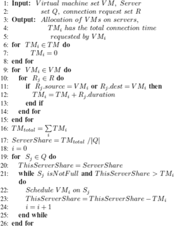

  

  Equal time distribution heuristic technique

• b) Node Distance Technique (ND):

  First, the average distance between each two nodes is calculated. The two nodes furthest from each other (with maximum distance) are chosen. Then, the maximum number of VMs is allocated on the servers of these two nodes. Next, the remaining nodes are evaluated, the node with maximum average distance to the previous two nodes is chosen. The same process is repeated until all the VMS are scheduled. The algorithm is described in pseudo code in Fig. 4. fillNode is a function that basically tries to schedule as many VMs as possible on the called node until the node’s resources are exhausted. fillNode is illustrated in Fig. 5.

  Fig. 4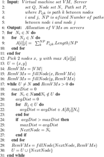

  

  Node distance heuristic technique

  Fig. 5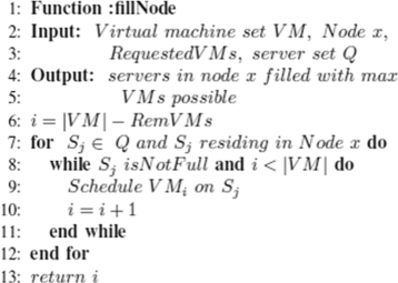

  

  Function: fillNode

• c) Resource Based Distribution Technique (RB):

  In this heuristic, the choice of the server is based on the type of VM requested. As shown in Table 3, three types of VMs are used in the experiment: i) High Memory Extra Large (MXL) has high memory configuration; ii) High CPU Extra Large (CXL) has a high computing power; iii) Standard Extra large (SXL) is more suited to typical applications that need a lot of storage space. Depending on the type of VM requested by the client, the heuristic picks the server with the highest amount of available corresponding resources. The VM then is allocated resources on that server. This causes the distribution to be more balanced.

Connection reservation heuristic techniques

• a) Duration Priority Technique (DP):

  In this heuristic, connections with the shortest duration are given the priority. First, connection requests are sorted based on the requested duration. The following step is to pick the connection with the shortest duration and schedule it on the shortest path available. This step is repeated until all connection requests are served. The algorithm is described in pseudo code in Fig. 6.

  Fig. 6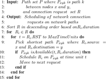

  

  Duration priority heuristic technique

• b) Greedy Algorithm (GA):

  In this heuristic, illustrated in Fig. 7, scheduling is based on the connection Requested Start Time (RST). Connection requests with earlier RST are scheduled on the first path available regardless of the path length.

  Fig. 7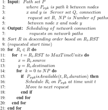

  

  Greedy heuristic technique

Complexity analysis of the heuristic solutions

The resource allocation problem in a cloud data center is a variation of the well known knapsack problem. The knapsack problem has two forms. In the decision form – which is considered less difficult - as it is NP-Complete- the question is: Can an objective value of at least K be achieved without exceeding a specific weight W? The optimization form of the problem – which is the form we try to solve in this work - tries to optimize the possible objective value. The optimization form is NP-Hard. This means it is at least as hard as all the NP problems. There is no current solution in polynomial time for this form.

This motivated the introduction of the heuristic algorithms. It might be of interest to the reader to visit the complexity of the introduced heuristic algorithms.

First, we revisit the variables covered in this analysis. VM represent the VM set, N represent the set of nodes, S is the set of servers, R is the set of connection requests, T is the allowed tardiness per request and D is the average duration of a connection. This analysis is offered with the sole purpose of being an approximation of the time complexity to show that these algorithms run within polynomial time and in turn- can be practically used by large scale cloud networks. Looking at the introduced algorithms one by one, we find that Equal time distribution has a complexity of O(|VM||R|+|S|). Node distance algorithms runs in O(|N ³|+|S|+|V|). Resource based distribution runs in O(|V||S|) which constitutes the quickest among the 3 VM placement algorithms we introduced. As for connection scheduling heuristics algorithms, Duration priority runs in O(|R|.lg|R|+|R|.T.D) or O(|R|.(1+lg|R|+T.D). Finally, the greedy connection scheduling algorithm runs in O(R.T.D). Therefore, all the mentioned algorithms run in polynomial times and can yield a result for large scale problem in practical time periods.

Suboptimal solution

Although an optimal solution can be obtained using the formulation in “Mathematical formulation” section, this is only feasible for small scale problems. Even when using a 5-node network with 4 servers and 7 links connecting them, the number of optimization variables can be as big as 5000 variables when scheduling 50 requests that belong to 5 VMs. On the other hand, heuristic methods achieve feasible solution in relatively quick times but the solution quality cannot be proven. This motivates us to move to the next step which is finding a method that achieves a suboptimal solution. The method introduced here is based on a decomposition technique. We illustrate the method in Fig. 8. The steps go as follows.

Fig. 8

The suboptimal method step by step

1- In Step 1, a set of known connection requests are preprocessed to generate interdependency measurements. This is figured out by calculating the frequency of communications between each two points in the network. To be more specific, the frequency of the connection requests between each VM _i and VM _j is calculated as well as the frequency of connection requests between VM _i and node _k which represent a private cloud. This gives us an indication of which direction most of the VM’s connections go. This is closely correlated with the dependencies this VM has and should ideally affect where it is scheduled.

2- In the second step, a utility function is constructed based on the connection frequency values generated in step 1. The utility function serves as the objective function of the master problem that allocates VMs on hosts.

3- Next, a master problem in which we handle the assignment of VMs to servers and connections to specific paths without scheduling them is generated. In other words, we solve for the decision variable X _vq without considering any scheduling constraints. This produces a feasible assignment for VMs that aims at scheduling interdependent VMs close to each other.

4- After getting the VM assignment locations, A subproblem in which we try to find the optimal scheduling for the input connections under these specific VM assignment conditions. In other words, we solve for the decision variable Y _ipw , F _i in the subproblem. The minimum tardiness produced from the subproblem is the objective value we are looking for. As in any decomposition based optimization, the success of the decomposition technique depends on the way the solution of the master problem is chosen. We formulate the master problem and the subproblem as follows.

Master problem formulation

We first introduce Distance function. It represents the distance between two nodes measured by the number of links in the shortest path between them. A frequency function based on connection duration is also added. This is a function where the connection duration is preferred as dominant factor. The frequency function is a value that will represent interdependency between two VMs or between a VM and a private cloud (client node). Another alternative here is depending on the number of connections requested between these two points rather than the total amount of connection time. Once we calculate the frequency function values, the utility function is constructed as:

$$ {}MIN \sum_{v \in VM}\sum_{u \in VM }\sum_{s \in Q}\sum_{q \in Q} ({Freq}_{vu}\times {Distance}_{sq}\times X_{vs}\times X_{uq}), $$

(12)

Subject to

$$ (2),(4). \qquad $$

(13)

The master problem finds the VM allocation that maximizes the value of point to point interdependency.

Subproblem

As the subproblem focuses on scheduling, its objective function is the same as in the optimal form, i.e., minimizing the average connection tardiness. In this case, the final value of the relaxed objective will come directly from the solution of the subproblem. The difference is that the subproblem already knows where the VMs are allocated and is scheduling connections accordingly. The objective of the sub-problem is as follows.

$$ MIN \sum_{i} (F_{i} - r_{i})\qquad\qquad i \in I, $$

(14)

Subject to

$$ (3),(5)-(11). \qquad $$

(15)

Results

Simulation environment

The problem is simulated using a discrete event based simulation program and solved on a more practical scale using the heuristic search techniques discussed in the previous sections. The network used for the experiment is the NSF network (in Fig. 9). It consists of 14 nodes of which 3 are data center nodes and the rest are considered client nodes [21]. Nodes are connected using a high speed network with a chosen link granularity that goes up to 3 lines (flows) per link. Fixed alternate routing method is used with 3 paths available between a node and any other node. Server configuration and request data parameters are detailed in Table 4. Preemption of connection requests is not allowed in this experiment.

Fig. 9

The NSF network of 14 nodes [29]

Table 4 Experiment parameter configuration

Heuristics

As explained in the previous sections, every experiment includes two phases and hence two heuristics are needed: one to schedule VMs on servers and the other to schedule connection requests. The five techniques explained earlier yield 6 possible combinations. However, We chose to show the results from the best 4 combinations (best 4 full-solutions). This is due to space constraints. The 4 chosen combinations cover all the 5 heuristics. The simulation scenarios and combined heuristics used for the two subproblems are as follows.

• 1-ED-GA: Equal Time Distribution technique and Greedy algorithm.

• 2-RB-DP: Resource Based Distribution technique and Duration Priority technique.

• 3-ED-DP: Equal Time Distribution technique and Duration Priority technique.

• 4-ND-DP: Node Distance technique and Greedy algorithm.

In Figs. 10 and 11, the 4 methods’ performances are compared in terms of the blocking percentage. This is measured as the request load increases. Figure 10 shows a comparison of the percentage of blocked requests (requests that could not be scheduled) where the allowed tardiness parameter value is very small (1 time unit). This means that this scenario resembles request requirements imposing close to real time scheduling. The x axis represents request load which is measured by λ/μ. λ represents the arrival rate and μ represents the service rate. Figure 11 shows the same comparison when the allowed tardiness per request is large (30000 time units). In both scenarios, it is noticed that ED-DP and RB-DP methods have shown a clear advantage by scoring consistently lower blocked requests. The common factor for these 2 methods is using DP to schedule connections. Therefore, this indicates a clear advantage of using DP over GA when scheduling connection requests in tight or real time conditions. In addition, As seen in Fig. 11, RB-DP has shown a decent advantage over ED-DP in terms of blocking percentage.

Fig. 10

Request Blocking results for scheduling methods (allowed tardiness/request =1 time units)

Fig. 11

Request Blocking results for scheduling methods (allowed tardiness/request =30,000 time units)

Regarding the other performance metric, average tardiness per request, the measurements are shown in Fig. 12. The figure shows a comparison of the average tardiness per request produced when using the four methods. Allowed tardiness in that experiment is small (25 time unit). Once more, ED-DP and RB-DP methods have shown a clear advantage by scoring consistently lower tardiness per request. Also, it is noticed from the figure the ED-DP produces slightly better results (less average tardiness) than RB-DP. Therefore, using RB-DP method is more suitable to scenarios where there is an emphasis on serving the largest number of requests. On the other hand, using ED-DP is more suitable to scenarios where the individual request performance or service level is prioritized over serving more requests.

Fig. 12

Request average tardiness results for scheduling methods (allowed tardiness/request =25 time units)

Relaxed solution results

With regards to the network we tested on, a 5-node network was used in these tests with 2 as data center nodes and the rest as client nodes (private clouds). Four servers were used in the tests with 2 servers in each data center. To connect the nodes in the physical network, 7 links were used and 20 different paths were defined. Two alternate routing paths were defined for each couple of nodes. The input contained data corresponding to 5 VM instances. The choice of this network is due to two factors. First, condensing requests in an architecture with limited resources puts the network under high load to eliminate the effect the network capacity would have on the result. This would allow more control by eliminating any factors related to network design or node distribution that might ease the pressure on the scheduling algorithm. This way, the problem size is controlled directly using only the parameters we are testing for which are the number of requests, their specification and their distribution. Second, it makes it easier to compare results and execution times of relaxed solution to those of the optimal solution.

For the connection requests coming from the clients, as in [22], their arrival rate values were set according to a Poisson process. The connection request lifetime (duration) was normally distributed with an average of 100 time units and the total number of connection requests was gradually increased from 20 up to 3000 requests. Every connection request is associated with a source, a destination, a requested start time and a duration. The source nodes/VMs were uniformly distributed.

To evaluate the optimal and relaxed solutions, we used the IBM ILOG CPLEX optimization studio v12.4. Both the optimal and relaxed solution were programmed using Optimization Programming Language (OPL) and multiple testing rounds were performed. Both solutions were tested for multiple values of normalized network load.

Table 5 shows a comparison between the objective values obtained using the optimal scheme vs. the values obtained from the relaxed (decomposed) scheme for small scale problems (up to 200 requests). While the optimal solution was able to schedule all requests without any delay (tardiness), the relaxed solution achieved an acceptable average tardiness in comparison. As noticed from the table, the execution times for the optimal scheme are slightly better for small data sets, but as the number of requests grows, the difference in execution times becomes evident. This goes on until the optimal solution becomes infeasible while the relaxed solution still executes in a relatively short period. The maximum number of requests the optimal solution is able to solve depends on the machines used and the network load parameters used to generate the input data.

Table 5 Optimal vs. relaxed solution values and execution times

Concerning large scale problems, the experimental results shown in Table 6 illustrate that the relaxed solution has achieved an acceptable average tardiness in comparison to the optimal solution. The effect of increasing the problem size on the value of average tardiness when using the relaxed solution is evident. The average tardiness achieved is less than 10% of the average request duration (lifetime). This is well within the bound set in [23] for acceptable connection tardiness which is half (50%) the lifetime or requested duration of the connection. This is also a considerable improvement over the performance of the heuristic solution which is shown in the same table (average tardiness values around 20% of request lifetime). The table also shows an increase in the average tardiness when increasing the number of requests (problem size). This is due to the fact that tardiness accumulates as priority is given to the request arriving earlier. In terms of execution time, as the number of requests grow, the difference in execution time between the optimal and relaxed solutions becomes evident. The optimal solution becomes infeasible while the relaxed solution still executes in a relatively short period scheduling 3000 requests in around in a period between 8–11 minutes depending on the network load.

Table 6 Execution times & average tardiness for connection requests for large scale problems when increasing the average connection duration to 100 Time units

To illustrate the impact of the allowed tardiness parameter on the request acceptance ratio, the results in Table 7 are presented. Using the heuristic solution with the combination RB-DP, the table shows the increase in the acceptance ratio as we increase the allowed tardiness per request for a specific network load.

Table 7 Connection requests acceptance rate for different network loads using the relxed solution

To measure the acceptance ratio, we introduced a maximum waiting period parameter (or allowed tardiness as discussed in previous sections). This parameter represents the period of time a connection request will wait to be served before it is considered blocked. For that, an ideal value is the same value used in [23], namely, half the request lifetime. In other words, If the connection waited for more than 50% of its duration and it was not scheduled then it is blocked or not served. Table 6 shows the acceptance ratio and the average tardiness for requests with an average duration of 100 time units.

Considering this scenario where requests with high tardiness are blocked presents a trade off between average connection tardiness and the percentage (or number) of blocked connections. It is noticed that the average tardiness decreases as we remove the requests with high tardiness and consider them blocked. An average tardiness of less than 2% of a request lifetime can be guaranteed if we are willing to sacrifice 13% of the requests as blocked.

Deciding weather to use this scenario or not is up to the cloud solution architects. This depends on the client sensitivity to the precision/quality vs. the speed of achieving results.

Comparison with previous solutions

When planning the comparison between the proposed solution and solutions available in the literature, we are faced with a challenge. As discussed in detail in “Related work” section, the available solutions are diverse in terms of the parameters considered and the covered dimensions of the cloud resource allocation problem. This limits the number of solutions that can realistically be used to solve this particular flavor of the problem. However, we were able to use the algorithms implemented in [6] (Modified best fit decreasing method) and [24, 25] (GREEN scheduling) to solve the same problem and compare their performance to the method we developed. The focus was: network capacity (minimizing blocking percentage) and performance (when blocking is not an issue, minimizing the average tardiness per served request is a priority). This comparison was performed for a smaller network first, in order to explore the stress effect on a cloud network. Then, the same comparison is performed for a larger more realistic network scenario. As in the previous experiments, the tests were performed for different problem sizes and various levels of allowed tardiness per requests.

Small network results

Figure 13 compares the three algorithms’ performance in terms of request blocking percentage for different scenarios as the allowed tardiness level increases. The figure shows that our technique (RB-DP) performs consistently better (lower blocking percentage) than Green scheduling algorithm. It also shows that RB-DP performs at the same level as MBFD for low allowed tardiness levels before showing an advantage for high allowed tardiness. Figure 14 presents results for the other metric, average request tardiness. Figure 14 shows that RB-DP starts by performing on the same level of the other two algorithms and while we increase the allowed tardiness level for requests, RB-DP shows clear advantage (as seen in the last case of allowed tardiness =1000 time units). The effect of increasing the allowed tardiness is basically eliminating the need to schedule each request as soon as it arrives (to avoid blocking requests) Instead, it focuses the experiment on showing the algorithm that can serve/schedule requests in the most efficient way and this, in turn, decreases the average tardiness per requests.

Fig. 13

Request blocking percentage results for 3 scheduling algorithms measured for 4 different allowed tardiness cases

Fig. 14

Request average tardiness results for 3 scheduling algorithms measured for 4 different allowed tardiness cases

Large network results

The same trends carry on while testing on large scale networks (the NSF network). In Fig. 15, blocking percentage is shown for the three algorithms for different problem sizes. Problem size here is represented by the number of requests submitted to the central controller per cycle (arrival rate). These results are shown for allowed tardiness level = 5 time units (very low level) which adds extra pressure to serve requests within a short period of their arrival and focuses the algorithms work on serving the highest number of requests not on tardiness levels. In Fig. 16, the same results are shown for a higher number of requests ranging from 3000 to 10,000 requests per cycle. This confirms that our experimental results are consistent when the network is exposed to higher load that is close to or exceeds its capacity. Looking at both figures, they show that our technique (RB-DP) performs consistently better than the other two algorithms under high loads.

Fig. 15

Request blocking percentage results for scheduling methods with allowed tardiness=5 units (very low)

Fig. 16

Request blocking percentage results for 3 scheduling algorithms for a large number of requests per cycle (1–10k)

Figure 17 explores the performance of the algorithms in the specific case of high allowed tardiness levels.

Fig. 17

Request blocking percentage results for scheduling methods while changing allowed tardiness levels

RB-DP offers clear advantage in terms of the blocking percentage metric for various allowed tardiness levels.

Moving to the second metric, Fig. 18 shows the performance of the three algorithms in terms of average request tardiness while changing the allowed tardiness levels (or request lifetime). RB-DP performs on a comparable level to the other two algorithms for small allowed tardiness levels and then exceeds the performance of MBFD starting medium levels of request lifetimes and then clearly exceeds both algorithms with the higher levels starting 400 time units.

Fig. 18

Request average tardiness results for scheduling methods (allowed tardiness/request =25 time units)

These results prove the potential our solution has in terms achieving better performance in both blocking percentage (more accepted connection requests and less network congestion) and average tardiness (better Quality of Service conditions for cloud users).

Conclusion

We introduced a comprehensive solution to tackle the problem of resource allocation in a cloud computing data center [26]. First, the problem was formulated as a mixed integer linear model. This formulation was solved using an optimization library for a small data set. However, finding the optimal solution for larger more practical scenarios is not feasible using the optimal mathematical formulation. Therefore, we introduced 5 heuristic methods to tackle the two sides of the problem, namely VM reservation and connection scheduling. The performance of these techniques was analyzed and compared. Although the solution scale issue is solved, a heuristic solution does not offer optimality guarantees. This constituted the motivation to introduce a suboptimal solution. The solution contained 4 steps that exploited the VM interdependency as a dominant factor in the VM allocation process. This allows us to solve the scheduling phase optimally in the following step which causes the solution to improve considerably. The relaxed solution achieved results matching with parameters preset in the literature for average connection tardiness. The results were also shown for the scenario where request blocking is allowed. Results were achieved without sacrificing the computational feasibility which shows our method to be a valid solution for reaching acceptable connection tardiness levels. Furthermore, the proposed solution was compared to two of the prominent algorithms in the literature. The proposed solution was shown to be advantageous in terms of minimizing both average request tardiness and blocking percentage for multiple cloud network scenarios. This makes it a strong candidate to be used in cloud scenarios where the focus is on metrics like more accepted connection requests and less network congestion or request average tardiness (better quality of service conditions for cloud users).

In the future, we plan to use our scheme to experiment with other important objectives of the cloud provider [27, 28]. Maintaining privacy while processing and communicating data through cloud resources is a critical challenge. Privacy is a major concern for users in the cloud or planning to move to the cloud. Improving data privacy metrics is not only important to clients, but also critical for conforming with governmental regulations that are materializing quickly. This means that a resource allocation system should extend its list of priorities to include privacy metrics in addition to typical performance and cost metrics. Constraints on the data handling, data movement and on scheduling locations should be seen. The privacy extends to data on resources required by the cloud clients. We have investigated some of the topic’s challenges at length in [3]. Our next step is to extend our model to explore these possibilities. This would add a different dimension to give a competitive advantage to cloud providers which offer the expected level of privacy to prospective clients.

References

Mckendrick J12 Most Memorable Cloud Computing Quotes from 2013, Forbes Magazine, [Online]. Available: https://www.forbes.com/sites/joemckendrick/2013/12/08/12-most-memorable-cloud-computing-quotes-from-2013/%237c88fe2330af. Accessed Feb 2017.
IBM’s The big data and analytics hub, The 4 Vs of the Big Data, IBM, [Online]. Available: http://www.ibmbigdatahub.com/infographic/four-vs-big-data. Accessed Feb 2017.
Abu Sharkh M, Jammal M, Ouda A, Shami A (2013) Resource Allocation In A Network-Based Cloud Computing Environment: Design Challenges. IEEE Commun Mag 51(11): 46–52.
Dastjerdi AV, Buyya R (2014) Compatibility-aware Cloud Service Composition Under Fuzzy Preferences of Users. IEEE Trans Cloud Comput 2(1): 1–13.
Wei G, Vasilakos AV, Zheng Y, Xiong N (2010) A game-theoretic method of fair resource allocation for cloud computing services. J Supercomput 54(2): 252–269.
Beloglazov A, Abawajy J, Buyya R (2012) Energy-aware resource allocation heuristics for efficient management of data centers for cloud computing. Futur Gener Comput Syst, Elsevier 28(5): 755–768.
Abu Sharkh M, Kanso A, Shami A, hln P (2016) Building a cloud on earth: a study of cloud computing data center simulators. Elsevier Comput Netw 108: 78–96.
Duan R, Prodan R, Li X (2014) Multi-objective game theoretic scheduling of bag-of-tasks workflows on hybrid clouds. IEEE Trans Cloud Comput 2(1): 29–42.
Guzek M, Kliazovich D, Bouvry P (2013) A holistic model for resource representation in virtualized cloud computing data centers In: proc CloudCom, vol. 1, 590–598.. IEEE.
Shojafar M, Cordeschi N, Baccarelli E (2016) Energy-efficient adaptive resource management for real-time vehicular cloud services. IEEE Trans Cloud ComputPP(99): 1rgy.
Cordeschi N, Shojafar M, Baccarelli E (2013) Energy-saving self-configuring networked data centers. Comput Netw 57(17): 3479–3491.
Shojafar M, Javanmardi S, Abolfazli S, Cordeschi N (2015) FUGE: A joint meta-heuristic approach to cloud job scheduling algorithm using fuzzy theory and a genetic method. Clust Comput: 1–16. http://link.springer.com/article/10.1007/s10586-014-0420-x.
Shojafar M, Cordeschi N, Abawajy JH (2015) In: Proc. of IEEE Global Communication Workshop (GLOBECOM) Workshop, 1–6.. IEEE.
IBMIBM CPLEX Optimizer [Online]. Available: http://www-01.ibm.com/software/commerce/optimization/cplex-optimizer/. Accessed Feb 2017.
Kantarci B, Mouftah HT (2012) Scheduling advance reservation requests for wavelength division multiplexed networks with static traffic demands In: proc. IEEE ISCC, 806–811.. IEEE.
Wallace TD, Shami A, Assi C (2008) Scheduling advance reservation requests for wavelength division multiplexed networks with static traffic demands. IET Commun 2(8): 1023–1033.
AmazonAmazon Elastic Compute Cloud (Amazon EC2), [Online]. Available: https://aws.amazon.com/ec2/. Accessed Feb 2017.
Maguluri S, Srikant R, Ying L (2012) Stochastic Models of Load Balancing and Schedulingin Cloud Computing Clusters In: proc. IEEE INFOCOM, 702–710.. IEEE.
Jammal M, Singh T, Shami A, Asal R, Li Y (2014) Software defined networking: State of the art and research challenges. Elsevier Comput Netw 72: 74–98.
Hawilo H, Shami A, Mirahmadi M, Asal R (2014) NFV: state of the art, challenges, and implementation in next generation mobile networks (vEPC). IEEE Network 28(6): 18–26.
Abu Sharkh M, Shami A, Ohlen P, Ouda A (2015) Simulating high availability scenarios in cloud data centers: a closer look In: 2015 IEEE 7th Int Conf Cloud Comput Technol Sci (CloudCom), 617–622.. IEEE.
Abu Sharkh M, Ouda A, Shami A (2013) A Resource Scheduling Model for Cloud Computing Data Centers In: Proc. IWCMC, 213–218.
Chowdhury M, Rahman MR, Boutaba R (2012) Vineyard: virtual network embedding algorithms with coordinated node and link mapping. IEEE/ACM Trans Netw 20(1): 206–219.
Kliazovich D, Bouvry P, Khan SU (2013) Simulation and performance analysis of data intensive and workload intensive cloud computing data centers. In: Kachris C, Bergman K, Tomkos I (eds)Optical Interconnects for Future Data Center Networks.. Springer-Verlag, New York. ISBN: 978-1-4614-4629-3, Chapter 4.
Kliazovich D, Bouvry P, Khan SU (2011) GreenCloud: a packet level simulator of energy-aware cloud computing data centers. J Supercomput 16(1): 65–75. Special issue on Green Networks.
Armbrust M, Fox A, Griffith R, Joseph A, Katz R, Konwinski A, Lee G, Patterson D, Rabkin A, Stoica I, Zaharia M (2009) Above the Clouds: A Berkeley View of Cloud Computing. Tech. Rep. UCB/EECS-2009–28. EECS Department, UC Berkeley.
Foster I, Zhao Y, Raicu I, Lu S (2008) Cloud Computing and Grid Computing 360-Degree Compared In: proc. GCE Workshop, 1–10.. IEEE.
Kalil M, Meerja KA, Refaey A, Shami A (2015) Virtual Mobile Networks in Clouds. Adv Mob Cloud Comput Syst: 165.
Miranda A, et al. (2014) Wavelength assignment using a hybrid evolutionary computation to reduce cross-phase modulation. J Microw Optoelectron Electromagn Appl 13(1). So Caetano do Sul http://dx.doi.org/10.1590/S2179-10742014000100001.
Acknowledgments
The authors would like to thank Dr. Rejaul Choudry for his contribution to the code implementation and related work section. The authors would also like to thank Dr. Daehyun Ban from Samsung for his insightful feedback.
Funding
This work is supported in part by the Natural Sciences and Engineering Research Council of Canada (NSERC-STPGP 447230) and Samsung Global Research Outreach (GRO) award.
Authors’ contributions
Dr. Mohamed Abu Sharkh reviewed the state of the art of the field, did the analysis of the current resource allocation techniques and their limitations. He formulated the problem in optimal and suboptimal forms, implemented the simulator presented in this paper, and performed the experiments as well as analysis. Prof. Abdallah Shami initiated and supervised this research, lead and approved its scientific contribution, provided general input, reviewed the article and issued his approval for the final version. Dr. Abdelkader Ouda provided general input and reviewed the article. All authors read and approved the final manuscript.
Competing interests
The authors declare that they have no competing interests.
Author information
Authors and Affiliations
Corresponding author
Rights and permissions
Open Access This article is distributed under the terms of the Creative Commons Attribution 4.0 International License(http://creativecommons.org/licenses/by/4.0/), which permits unrestricted use, distribution, and reproduction in any medium, provided you give appropriate credit to the original author(s) and the source, provide a link to the Creative Commons license, and indicate if changes were made.
About this article
Cite this article
Abu Sharkh, M., Shami, A. & Ouda, A. Optimal and suboptimal resource allocation techniques in cloud computing data centers. J Cloud Comp 6, 6 (2017). https://doi.org/10.1186/s13677-017-0075-2
Received:
Accepted:
Published:
DOI: https://doi.org/10.1186/s13677-017-0075-2