Double auction and profit maximization mechanism for jobs with heterogeneous durations in cloud federations

Abstract

By sharing resources with each other, different cloud providers in a cloud federation can exploit their diversity in resource configuration and operational cost so as to improve service performance. They should consider the strategy of resource pricing, job scheduling and server provisioning altogether to maximize their own interests. On the other hand, they need to efficiently trade the resources with a suitable mechanism, typically auction, so as to guarantee the participants’ profits. Nevertheless, in consideration of the heterogeneous execution times of jobs, both the pricing strategy and trading mechanism should be delicately designed, which is obviously a challenging task. In this paper, we firstly propose a truthful, individual-rational and ex-post budget-balanced auction mechanism for selecting pairs of buyer and seller winners to trade virtual machines for different durations. Then, to maximize the individual profits, we propose a dynamic resource bidding scheme and a job scheduling strategy based on our importance model of jobs with heterogeneous execution times and resource requirements. The simulation results show that, compared with existing ones, our design can better handle varieties of both execution time and resource requirement and make the participants obtain more individual profits.

Introduction

Cloud computing is nowadays the predominant paradigm for large scale information systems, especially Internet applications, more and more clouds are established around the world. To improve cloud resource utility, cloud federation [1] has emerged as a new technology/paradigm to enable resource sharing among different clouds owned by different cloud service providers.

By sharing resources with each other, cloud providers in the federation can exploit their difference in resources and diversity in user demands, so as to improve service quality and save resource investment. Since workloads are unpredictable, tremendous and bursty [2, 3], a cloud may elastically lease resources, usually VMs, from other clouds, so as to cope with the load peak and avoid the risk of losing customers and long term revenue due to performance degradation. Therefore, federation offers participants the opportunity to obtain more profits from the temporal and geographical diversity among different clouds [4], because both resource utilization and individual profits can be potentially improved.

However, resource sharing among clouds in a federation is not a travail issue in terms of mechanism design and deployment, because different clouds and different users are involved, which all have different resources and requirements. Considering profits of different participants, it is hard to get the optimal solution.

Auction is an efficient mechanism widely adopted in resource trading mechanism for cloud computing environments [5, 6], especially cloud federations [7–9]. In a cloud resource auction, cloud providers offer resources to cloud users. Since there are multiple sellers and multiple buyers, double auction, instead of single auction, is usually used for resource trading in cloud federation [9]. A double auction refers to an auction with both multiple buyers and multiple sellers are involved in trading simultaneously.

Many auction based mechanism and algorithms have been proposed for resource trading in cloud federations and a comprehensive survey can be found in [9]. Most of these works aim to maximize the social welfare of the whole federation [1, 9–12], and four major properties are expected to hold:

• Truthfulness: an auction mechanism is said to be truthful if disclosing the private valuation truthfully is always the dominant strategy for a seller or buyer to get an optimal utility, no matter what strategies are used by other participants.

• Computational efficiency: the auction outcome (allocation of resources and calculation of clearing price and payment) should be computed in polynomial time.

• Budget balance: all monetary transfers must be done between cloud buyers and the cloud sellers, and the auctioneer or broker (a trust worthy third party who supervise the auction) should not lose or gain money.

• Individual rationality: a seller is always paid no less than the price of a resource offered by a provider, and a buyer always pays no more than its bid, i.e., the price at which the buyer is willing to buy the resource.

Besides the social welfare of the federation, maximizing the profit of individual participant in resource trading of cloud federation has also been considered. Most of these works focus on the pricing policies/mechanisms [13–15]. The double auction mechanism proposed by Li et al. [4] should be the only solution, to the best of our knowledge, that can achieve the optimal individual profit over the long run in a cloud federation. Other works can only guarantee individual rationality, nonnegative profit gain.

However, the auction mechanism in [4] is limited by its assumption of single timeslot duration of all jobs, i.e., VM requests. In practice, different jobs may have different time durations, while the solution in [4] cannot handle such heterogeneity.

On the one hand, the multi-timeslot nature leads to the potentially increased job types, perplexing the scheduling decision. On the other hand, once a job is scheduled, it will run continuously until completed, which means VM resources should not only be leased for a single timeslot either.

Motivated by the above issues, we propose a new double auction based resource trading and scheduling solution. We design new auction mechanism and associated strategies, including pricing, scheduling and provisioning decision to handle bids of resources with multi-timeslot.

More precisely, the contributions of this work are summarized as follows.

• We design a double auction-based mechanism that can select pairs of buyer and seller winners to trade virtual machines for different durations. The auction is also in line with personal rationality and ex-post-budget balance while guaranteeing the participants to bid truthfully. Through this auction mechanism, each cloud can trade different types of resources in each timeslot, which enables each winner cloud to rent them for a desirable duration and a specified amount of resources as far as possible.

• We propose the objective function of maximizing individual profits for clouds and model the jobs with heterogeneous durations and required resources in a consistent form. Considering the auction mechanism and the revenue target of each cloud, we use the Lyapunov method to acquire the corresponding pricing strategy, so that each cloud maximizes its winning probability and ensures its benefit as well. In order to maximize the profits, we have designed pertinent scheduling algorithms to make full use of resources and provide an adequate quantity of servers.

Related work

Early works on cloud resource allocation focus on improving resource utilization and saving energy in a single cloud [16, 17]. With the further development of cloud computing, a cloud provider may have several clouds, and cloud resource allocation for multiple clouds are studied. Sun et al. propose a novel multi-layered scheduling architecture to improve resource utilization by speculate over-subscription and rescheduling strategies [18]. Zhao et al. search the equilibrium point of supply-demand relationship to better pricing its resources in geo-distributed data centers and propose corresponding scheduling rule to maximize profit [19]. Mashayekhy et al. capture the incentives of the users by auction-based online mechanism to dynamically price its resources for them and strategically allocate resources to obtain higher profit [20]. Taking both computational resources and communication resources into consideration, Shi et al. propose SWMOA to price virtual clusters dynamically and PROMA to maximize revenue [21]. Li et al. propose a truthful online auction mechanism for profit maximization and handle time-varying user demands with an elastic model [22].

To better determine resource prices in cloud networking systems, the auction mechanism is increasingly widely used, which is observed by Luong et al. [23] and various related economic methods are surveyed. However, the clouds in these works still belong to an autonomous enterprise and share intergrated information to make pricing and scheduling decisions

Different from these studies on clouds with centralized control, resource sharing in cloud federations has been recently considered and studied. Most of them adopt double auction based mechanism and aim to maximize the social welfare of the whole federation.

Tang et al. [10] consider multi- resource fairness among the individual clouds in a federation in a long term to achieve a higher resource utilization rather than revenue. Ye et al. [11] focus on resource utilization of the federation by a reinsurance- emulated retention share strategy instead of profit maximization. Ray et al. [1] propose a cloud federation formation mechanism based on hedonic coaliton game where the clouds cooperate to minimize migration cost and obtain more profit for the federation.

Kumar et al. [9] propose a multi-unit double auction based mechanism, called TMDA, the first one being truthful for both the cloud users and the providers. TMDA is also individual rational, budget-balance. Kumar et al. [24] also propose a truthful combinatorial double auction mechanism for allocation and pricing of computing resources in cloud. For resource allocation, utilitarian social welfare maximization problem is formulated using Integer Linear Programming (ILP) and a near optimal solution is obtained using Linear Programming based padded method.

Middya et al. [12] propose a multi-unit double auction mechanism for users to efficiently choose cloud federations from which they can get resources. The authors consider a multi-seller and multi-buyer double auction mechanism for heterogeneous resources, where every buyer submits their bids and every seller places their offers.Besides maximization of social welfare of the whole federation, researchers have considered individual profit maximization recently, i.e. they attempt to maximize the profit of individual users and clouds.

Zant et al. [14] consider various types of pricing policies, including on-demand, spot, reserved, etc. and conduct simulations to evaluate their performance. Zhang et al. [15] propose effective pricing functions for a cloud provider to employ, for computing unit resource prices at each time point. The computed prices are posted as ‘take it or leave it’ prices for cloud users to decide whether to rent the cloud resources, while users’ job valuations are not revealed to the cloud provider. Such prices can also serve in a posted-price auction mechanism for cloud job admission and charging. Wei et al. [13] propose a Stackelberg game among the clouds to decide their own posted prices to trade more resources to users instead of to other clouds.

Li et al. [4] investigate VM trading in a federation of selfish clouds, each aiming at maximizing its own profit by serving more job requests and selling its resource in a higher prices. A double-auction-based mechanism is proposed for the sell and purchase of available VMs across cloud boundaries over time. Moreover, an efficient dynamic VM trading and scheduling algorithm is proposed to decide the true valuations of VMs in the auction, and schedule arriving jobs with different number of VMs and SLAs. The algorithm can also judiciously turn on and off servers in the clouds based on the current electricity prices. The dynamic algorithm serves as an efficient strategy for each cloud to employ in the online double auction. Different from other works on auction mechanism, the solution in [4] has two major advantages: i) it explicitly addresses individual profit maximization over the long run (other works provide only individual rationality, i.e., nonnegative profit gain), ii) it provides methods to quantitatively calculate the true valuations in each bid (which is usually assumed to be known in other works). At the same time, this solution has all desirable properties such as truthfulness, ex-post budget balance, and social welfare maximization.

Our work also focuses on individual profit maximization for selfish clouds in federation, and we extend the problem studied in [4] by considering heterogeneous job durations. More precisely, the problem formulated in [4] considers jobs with only one timeslot, which is obviously not always true in practice. Jobs from users are diverse and may last for multiple timeslots. We design a novel auction mechanism and modify the job importance model to make up its shortcoming. We also propose corresponding job scheduling and server provisioning strategies to maximize individual profit of each cloud.

System model and problem formulation

The cloud

We consider a federation with a number, denoted by F, of clouds distributed in different locations, each of which operates autonomously to maximize self-interest by intelligently serving its own customers’ job requests, managing local servers and trading resources with other clouds.

Each cloud i∈{1,...,F} can serve S types of jobs, each of which is specified by a five-tuple 〈m_s,g_s,l_s,d_s,v_s〉. Here, m_s∈{1,...M} specifies the type of the required VM instances of job type s∈{1,...,S}, where M is the maximum number of VM types, and each type corresponds to a different CPU to memory ratio; g_s is the number of type m_s VMs that the job needs simultaneously; l_s∈{1,...,L} and d_s stands for the execution time and the service level agreement (SLA); and v_s shows the data volume processed by type s jobs.

Each cloud runs in a timeslotted fashion. At the beginning of each timeslot t, a lot of job requests are submitted to cloud i, and $r_{i}^{s}(t) \in \{0,...,R_{i}^{s}\}$ requests for each job type s are accepted. $R_{i}^{s}$ is the upper bound of the quota for accepting type s job in a timeslot. The process is illustrated in Fig. 1.

Fig. 1

The process in cloud i

The accepted jobs wait in FIFO queues for scheduling. $p_{i}^{s}(t)$ is the imprest paid by customers when committing a type s job to cloud i in timeslot t, which covers the resource usage fee and so on. For each timeslot, cloud i may schedule some jobs to VMs owned by itself or leased from other clouds, to avoid drop penalty. Let $\mu _{ij}^{s}(t)$ represents the number of type s jobs of cloud i scheduled for processing in cloud j at the beginning of timeslot t. To process in other clouds, the local data required by the jobs should be transmitted to target clusters, resulting in the transmission cost δv_s, where δ is the transmission cost for each unit of data volume. Cloud i will also drop $D_{i}^{s}(t)$ type s jobs according to its current condition and compensate the customers at a price $\xi _{i}^{s}$, which is no less than the fee charged to them when accepting the jobs, i.e., $\xi _{i}^{s} \ge p_{i}^{s}(t_{a})$, where t_a is the commit time of the jobs. For $D_{i}^{s}(t)$, we have

$$ D_{i}^{s}(t) \in \left\{0,...,D_{i}^{s(max)}\right\}, $$

(1)

where $D_{i}^{s(max)}$ is the upper bound of $D_{i}^{s}(t)$. Considering these actions, we can model the FIFO queue of type s jobs in cloud i as

$$\begin{array}{*{20}l} W_{i}^{s}(t\! +\! 1)\! \! =\! \! max\! \left\{\! W_{i}^{s}(t)\! -\! \sum\limits_{j=1}^{F} \mu_{ij}^{s}(t)\right. \! - &\left.\! D_{i}^{s}(t), 0{\vphantom{\sum\limits_{j=1}^{F} \mu_{ij}}}\right\} + r_{i}^{s}(t) \\ \forall s \in \{1,...,S\} \end{array} $$

(2)

Considering the required VM volume and estimated execution time, we further model the importance of unscheduled type s job requests in cloud i as

$$\begin{array}{*{20}l} & Q_{i}^{s}(t\! +\! 1)\! = \! max\! \left\{\! Q_{i}^{s}(t) \! -\! \sum\limits_{j=1}^{F} l_{s} g_{s} \mu_{ij}^{s}(t) - l_{s} g_{s} D_{i}^{s}(t), 0\right\} \\ & + l_{s} g_{s} r_{i}^{s}(t) \qquad \qquad \qquad \qquad \forall s \in \{1,...,S\} \end{array} $$

(3)

$Q_{i}^{s}$ will be 0 when the FIFO queue of type s job is empty, i.e., when all the type s jobs in cloud i are served or dropped, and no new jobs arrive. Since all the jobs should be scheduled or dropped to avoid SLA violation, we model the urgency by applying the ε-persistence queue technique [25] in a virtual queue $Z_{i}^{s}, \forall i \in \{1,...,F\}$, such that

$$ \begin{aligned} &Z_{i}^{s}(t\! +\! 1) \! =\! max\! \left\{\! Z_{i}^{s}(t) \! + \mathbf{\! 1}_{\left\{Q_{i}^{s}(t)>0\right\}}\! \cdot\! \left[\! \epsilon_{s} \! -\! \sum\limits_{j=1}^{F} \! l_{s} g_{s} \mu_{ij}^{s}(t)\right]\right. \\ &\left. - l_{s} g_{s} D_{i}^{s}(t) \! - \! \mathbf{1}_{\left\{Q_{i}^{s}(t)=0\right\}} l_{s} \sum\limits_{j=1}^{F} C_{j}^{m_{s}} N_{j}^{m_{s}},0 \right\} \! ~\forall s \in \! \{1,...,S\} \\ \end{aligned} $$

(4)

$$ \begin{aligned} &\mathbf{1}_{\left\{Q_{i}^{s}(t)>0\right\}} = \left\{ \begin{aligned} &1, \quad if \ Q_{i}^{s}(t) > 0 \\ &0, \quad otherwise \end{aligned} \right. \\ &\mathbf{1}_{\left\{Q_{i}^{s}(t)=0\right\}} = \left\{ \begin{aligned} &1, \quad if \ Q_{i}^{s}(t) = 0 \\ &0, \quad otherwise \end{aligned} \right.\\ \end{aligned} $$

Here, ε_s>0 is a constant and it makes $Z_{i}^{s}$ accumulate as time goes by when the type s job queue is not empty. Thus, the length of this virtual queue approximately reflects the accumulated response delay of jobs from the respective job queue. When the job queue is empty, the accumulated response delay is reduced with $l_{s} \sum \limits _{j=1}^{F} C_{j}^{m_{s}} N_{j}^{m_{s}}$. By modifying ε_s, we are able to bound the lengths of the queues and hence the maximum response delay can be bounded, i.e., the SLA constraint is satisfied [4].

During job execution, the jobs continuously occupy the required VM resources and generate the operational cost β_i(t) for running a server in cloud i, which mainly consists of electricity cost. Cloud i has $N_{i}^{m}$ homogenous servers to provision VMs of type m∈{1,...,M}, each of which can provide a maximum of $C_{i}^{m}$ VMs of its type. Let $n_{i}^{m}(t)$ be the number of active servers provisioning type m VMs at cloud i in t. The feasible job scheduling at time t is constrained by active servers and their capabilities, i.e.,

$$ n_{i}^{m}(t) \le N_{i}^{m} \qquad \forall m \in \{1,...,M\} $$

(5)

$$ \begin{aligned} \sum\limits_{s:m_{s}=m,s \in \{1,...,S\}}\sum\limits_{\tau = t-l_{s}}^{t}\sum\limits_{j=1}^{F} g_{s} \mu_{ji}^{s}(\tau) \le & C_{i}^{m} \cdot n_{i}^{m}(t) \\ \forall m \in \{1,...,M\} \end{aligned} $$

(6)

Equation (5) ensures that the number of active type m servers cannot exceed the total number of avaiable type m servers at each cloud. Equation (6) points out that the required number of type m VMs of unfinished jobs and newly scheduled jobs from cloud i itself and others should be within the capacity of corresponding active servers.

Virtual machine trading in cloud federation

As a federation, clouds are willing to cooperate with each other while as individual entities, they concern their own benefits. Under normal circumstances, for high load clouds, they may need more VMs to avoid dropping too many jobs and the low load ones may have idle VMs on sale. In fact, only if the price is reasonable, the clouds will also sell the resources regardless of the workload condition to maximize their economic benefits. Since there are generally more than one buyer and one seller, a double auction mechanism is naturally suitable for implementing efficient trading in this case, allowing both buying and selling clouds to actively participate in pricing, on behalf of their own benefits. In our dynamic systems, a multi-unit double auction is carried out among the clouds at the beginning of each timeslot.

In an auction, there are three roles for the participants.

Buyers and Sellers: A cloud can be both a seller and a buyer. A buy bid $\langle b_{i}^{m}(t),\alpha _{b,i}^{m}(t), \iota _{b,i}^{m}(t) \rangle$ records the unit price, maximum quantity and longest lease time, at which cloud i is willing to buy VMs of type m in t. Similarly, $\langle s_{i}^{m}(t), \alpha _{s,i}^{m}(t), \iota _{s,i}^{m}(t) \rangle$ is a sell bid. The buy and sell bids will be sent to the auctioneer at the beginning of timeslot t.

Let $\tilde {b}_{i}^{m}(t)$ and $\tilde {s}_{i}^{m}(t)$ be cloud i’s true valuation of buy price and sell price for a type m VM respectively. Similarly, let $\tilde {\alpha }_{b,i}^{m}(t)$ and $\tilde {\alpha }_{s,i}^{m}(t)$ be cloud i’s true valuation of the maximum volume of VMs it willing to purchase or sell. Also, let $\tilde {\iota _{b,i}^{m}(t)}, \tilde {\iota _{s,i}^{m}(t)}$ be cloud i’s true valuation of the maximum duration it willing to purchase or sell such volume of VMs. Aiming at maximizing its own profit, a cloud may cheat in bidding. To avoid this, we propose a truthful double auction mechanism in “Double auction mechanism” section, which guarantees the cheaters won’t obtain more profits than bidding honestly.

Auctioneer: We assume that there is a broker, acting as an auctioneer in the cloud federation. After collecting all the buy and sell bids, the auctioneer carries out the double auction in “Double auction mechanism” section to decide the buyer and seller winners, their deal prices and the upper bound of the quantities of VMs to trade in each VM type m. Let $\hat {b}_{i}^{m}(t)$ and $\hat {s}_{i}^{m}(t)$ be the deal prices for cloud i to buy and sell a type m VM respectively. The buyer will determine final purchase quantity of VMs and corresponding lease periods, constrained by their upper bounds.

Let $\alpha _{ij}^{m,l}(t)$ be the number of type m VMs that cloud i purchases from cloud j for l slot(s) since t, ∀i,j∈{1,...,F},i≠j.

$$ \alpha_{ij}^{m}(t) = \sum\limits_{l = 1}^{L} \alpha_{ij}^{m, l}(t) \qquad \forall m \in \{1,...,M\} $$

(7)

$$ \hat{\gamma}_{i}^{m}(t) = \sum\limits_{j \ne i} \sum\limits_{l = 1}^{L} l \alpha_{ij}^{m, l}(t) \qquad \forall m \in \{1,...,M\} $$

(8)

$$ \hat{\eta}_{i}^{m}(t) = \sum\limits_{j \ne i} \sum\limits_{l = 1}^{L} l \alpha_{ji}^{m, l}(t) \qquad \forall m \in \{1,...,M\} $$

(9)

$\hat {\gamma }_{i}^{m}(t)$ is the real quantity and corresponding duration of VMs purchasing from other clouds in timeslot t and $\hat {\eta }_{i}^{m}(t)$ is the quantity and duration selling to other clouds.

Since VMs are purchased for serving jobs, the job scheduling decisions $\mu _{ij}^{s}(t)$ at each cloud i∈{1,...,F} are constrained by the number of VMs it purchases

$$\begin{array}{*{20}l} & \sum\limits_{s:s\in\{1,...,S\}, m_{s} = m, l_{s} = l} g_{s} \mu_{ij}^{s}(t) = \alpha_{ij}^{m, l}(t) \\ & \forall m \in \{1,...,M\}, \\ &\forall l \in \{1,...,L\},\\ &\forall i,j \in \{1,...,F\}, i \ne j \end{array} $$

(10)

To make the auctioneer’s mechanism practical, three economic properties are required. 1) Truthfulness: Both bidder strategies and auction design will be simplified if bidding true valuation is a dominant strategy for the participants. 2) Individual Rationality: Only if each cloud is able to obtain a nonnegative profit from the auction, they will participate in it. 3) Ex-post Budget Balance: The auctioneer won’t host the aution unless it has a nonnegative surplus, i.e., the total payment from the buy winners is no less than the total charge asked by the seller winners in each timeslot.

Individual profit definition

Each cloud in the federation aims at maximizing its time-averaged profit over the long run, while trying to satisfy the resource and SLA requirements of each job.

Income: A cloud can earn income in two ways: 1) to charge customers for serving their job requests and 2) to sell VM resources to other clouds. The time-averaged income of cloud i∈{1,...,F} from serving their job requests is

$$ \Phi_{1}^{i} = {\lim}_{T\rightarrow\infty} \frac{1}{T} \sum\limits_{t=0}^{T-1} \sum\limits_{s=1}^{S} \mathbb{E} \{p_{i}^{s}(t)\cdot r_{i}^{s}(t)\} $$

(11)

We assume the charges $p_{i}^{s}(t)$ of service s∈{1,...,S} in each timeslot t are given. Since the arriving rates $r_{i}^{s}(t)$ are determined by the number of job requests accepted at the beginning of timeslot t, this part of income can be regard as fixed in each time.

The time-averaged income of cloud i∈{1,...,F} from selling VM resources is

$$ \Phi_{2}^{i} = {\lim}_{T\rightarrow\infty} \frac{1}{T} \sum\limits_{t=0}^{T-1} \sum\limits_{m=1}^{M} \mathbb{E} \{\hat{s}_{i}^{m}(t) \cdot \hat{\eta}_{i}^{m}(t)\} $$

(12)

Cloud i can increase this income by strategically proposing sell bids, i.e., $s_{i}^{m}(t), \alpha _{s,i}^{m}(t)$ and $\iota _{s,i}^{m}(t) (\forall m \in \{1,...,M\})$, at each time. Although $\alpha _{s,i}^{m}(t)$ is not directly related to this income, a larger $\alpha _{s,i}^{m}(t)$ somehow indicates a larger $\mu _{ji}^{s}(t)$, which raises this income potentially.

Cost: A cloud has four kinds of expenditure: 1) the operational cost of active servers, which mainly consists of electricity cost, 2) the payment of buying VM resources, 3) the transmission cost of delivering data to other clouds when scheduling jobs to them, and 4) the penalty for dropping jobs. The time-averaged operational cost of active servers of cloud i∈{1,...,F} is

$$ \Psi_{1}^{i} = {\lim}_{T\rightarrow\infty} \frac{1}{T} \sum\limits_{t=0}^{T-1} \sum\limits_{m=1}^{M} \mathbb{E} \{\beta_{i}(t)\cdot n_{i}^{m}(t)\} $$

(13)

which is generated by the active servers in each timeslot. The time-averaged payment of buying VM resources of cloud i∈{1,...,F} is

$$ \Psi_{2}^{i} = {\lim}_{T\rightarrow\infty} \frac{1}{T} \sum\limits_{t=0}^{T-1} \sum\limits_{m=1}^{M} \mathbb{E} \{\hat{b}_{i}^{m}(t)\cdot \hat{\gamma}_{i}^{m}(t)\} $$

(14)

Similar to $\Phi _{2}^{i}$, cloud i can reduce this expenditure by adjusting its buy bids, i.e., $b_{i}^{m}(t), \alpha _{b,i}^{m}(t)$ and $\iota _{b,i}^{m}(t) (\forall m \in \{1,...,M\})$, at each time. The time-averaged cost for transmitting data of cloud i∈{1,...,F} is determined by the data volume and number of jobs scheduling to other clouds, i.e.,

$$ \Psi_{3}^{i} = {\lim}_{T\rightarrow\infty} \frac{1}{T} \sum\limits_{t=0}^{T-1} \sum\limits_{s=1}^{S} \mathbb{E} \{\delta v_{s} \sum\limits_{j \ne i} \mu_{ij}^{s}(t)\} $$

(15)

The time-averaged penalty for dropping jobs of cloud i∈{1,...,F} is related to the volume of dropped jobs, i.e.,

$$ \Psi_{4}^{i} = {\lim}_{T\rightarrow\infty} \frac{1}{T} \sum\limits_{t=0}^{T-1} \sum\limits_{s=1}^{S} \mathbb{E} \{\xi_{i}^{s} \cdot D_{i}^{s}(t)\} $$

(16)

Profit Maximization: The profit maximization problem at cloud i∈{1,...,F} can be formulated as follows:

$$ \begin{aligned} \max & \qquad \Phi_{1}^{i} + \Phi_{2}^{i} - \Psi_{1}^{i} - \Psi_{2}^{i} - \Psi_{3}^{i} - \Psi_{4}^{i} \\ & \text{s.t. Constraints} \quad (1), (5) - (10) \end{aligned} $$

(17)

Cloud information notations are summarized in Table 1.

Table 1 Cloud Information Notation

Double auction mechanism

Overview

During each timeslot, the entire VM trading framework is depicted in Fig. 2, and works as follows.

• Step 1: Each cloud evaluates its true valuations of sell prices, buy prices and corresponding volume of different types of VMs, and submits them to the auctioneer.

  Fig. 2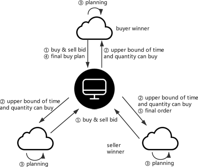

  

  Overview of the double auction mechanism

• Step 2: After collecting the bids, the auctioneer executes the double auction to determine the seller and buyer winners in the current round.

• Step 3: The actual valuations of buy and sell prices ofzthe winners are decided by the auctioneer, and the upper bounds of VM volume to trade are also given by it.

• Step 4: Based on the auction result, the buy winners reports the actual buying VM volume to the auctioneer and the auctioneer finally sends the actual selling VM volumes to the sell winners respectively.

• Step 5: Each cloud makes its job scheduling and server provisioning plan according to the transaction result.

Our double auction mechanism is used in Step 2 - 4 to decide winners, auction and to release result.

Three phases of double auction mechanism

We firstly design a double auction mechanism which can select pairs of buyer and seller winners to trade virtual machines for different durations for inter-cloud VM trading. Auction related notations are summarized in Table 2.

Table 2 Auction Related Notations

After collecting the bids from all clouds in the federation, the auctioneer carries out the following mechanism to decide the actual trading price for each type of VMs.

1) Determining Winners and Pairing: This phase is carried out in Step 2 of the auction mechanism. Firstly, the auctioneer discards bids from the clouds whose sell bid price is lower than its buy bid price. Then it sorts the remaining buy (sell) bids in non-ascending (-descending) order by the buy (sell) prices, and if the prices are the same, sorts them by durations in descending order. Let us denote the ordered buy prices for type m VM as $\lambda _{1}^{m}(t), \lambda _{2}^{m}(t),..., \lambda _{F}^{m}(t)$, and sell prices as $\zeta _{1}^{m}(t), \zeta _{2}^{m}(t),..., \zeta _{F}^{m}(t)$. The auctioneer then traverses the sequence until $\lambda _{k}^{m}(t) < \zeta _{k}^{m}(t)$. If k>2, then the clouds whose buy price (sell price) ranking from [1,k−2] are buyer (seller) winners, as illustrated in Fig. 3 (b), where k=5 and 3 pairs of winners are selected. On the contrary, no cloud win if k≤2.

Fig. 3

Determining Winners and Pairing. We only show cloud ID, bid price and duration here. E.g. (0,10,2) stands for cloud 0 bidding price $10 and duration 2 timeslots

We match the buyer and seller winners according to different durations. We again sort the winners’ bids by durations in a descending order. Although intuitively simply match them one by one is applicable, it may result in that no paricipants are fully satisfied. For example, the request of buyer winners requesting for 5, 3, 2 timeslots will match the seller winners offering 3, 2, 1 timeslots respectively, such that all the buyer winners can only buy resources for their less important jobs or even buy none.

Therefore, for each buyer winner, we choose to match it to the first unmatched seller winner whose $\iota _{s,i}^{m}(t)$ is not shorter than the buyer’s requirement, i.e., $\iota _{b,j}^{m}(t)$. As a result, if a buyer winner’s requirement is longer than the offer of all seller winners, it cannot buy any resource, as shown in Fig. 3 (c). What’s more, the k−1 buyer can become a buyer winner if it has the same bid price as an unmatched buyer winner and its time request can pair an unmatched seller winner. As illustrated in Fig. 3 (d), Cloud 6’s bid price is equal to Cloud 2, while its request time can match with Cloud 5, so it becomes the winner and Cloud 2 loses. After the adjustment, more buyer winners can be paired with their best matched seller winners. If a cloud is finally paired with itself, it is judged to lose.

2) Determining Deal Price and Volume Upper Bound: This phase is carried out in Step 3 of the auction mechanism. When k>2, let $P = \frac {\lambda _{k-1}^{m}(t) + \zeta _{k-1}^{m}(t)}{2}$. The price charged to each buyer cloud i of type m VMs is

$$ \begin{aligned} \hat{b}_{i}^{m}(t) = \left\{ \begin{aligned} &P, \quad \text{if \ bid } b_{i}^{m}(t) \text{ wins}\\ &0, \quad \text{otherwise} \end{aligned} \right.\\ \end{aligned} $$

(18)

The price paid to each seller cloud i of type m VMs is

$$ \begin{aligned} \hat{s}_{i}^{m}(t) = \left\{ \begin{aligned} &P, \quad \text{if \ bid } s_{i}^{m}(t) \text{ wins}\\ &0, \quad \text{otherwise} \end{aligned} \right.\\ \end{aligned} $$

(19)

To ensure each buyer and seller winner can be involved in the transaction, we match them in pairs, i.e., the buyers bidding $\lambda _{\kappa }^{m}(t)$ buy VMs from the sellers bidding $\zeta _{\kappa }^{m}(t) (\forall \kappa \le k - 2)$. Therefore, the upper bound of purchasing volume of each buyer cloud i can be determined as

$$ \begin{aligned} \overline{\alpha}_{ij}^{m}(t) = \left\{ \begin{aligned} \alpha_{s,j}^{m}(t), &\quad \text{if buyer } {i} \text{ matches with seller {j}} \\ 0, &\quad \text{otherwise} \end{aligned} \right.\\ \end{aligned} $$

(20)

Then, these values will be sent to corresponding clouds to help them make their final scheduling decisions at time t.

3) Announcing Result: This phase is carried out in Step 4 of the auction mechanism. When the final scheduling decision is made, each buyer cloud i will submit the final purchasing volume $\hat {\alpha }_{ij}^{m,l}(t)$ and corresponding lease period $l (l \le \iota _{s,j}^{m}(t))$, adding up to $\hat {\alpha }_{ij}^{m}(t)$, which is restricted by the upper bound. Then $\hat {\gamma }_{i}^{m}(t)$ is determined. The auctioneer will notify the corresponding seller clouds with the values as the final selling volumes and corresponding durations. And $\hat {\eta }_{j}^{m}(t)$ can be obtained at the same time.

Properties of the double auction mechanism

We now show that our double auction mechanism can meet the requirement of economic properties specified at the end of “Virtual machine trading in cloud federation” section.

Proof of truthfulness

Lemma 1.

(Monotonic Winner Determination) Given prices of buy bids $\{b_{1}^{m}(t),..., b_{i}^{m}(t),..., b_{F}^{m}(t)\}$ and sell bids $\{s_{1}^{m}(t),..., s_{i}^{m}(t),..., s_{F}^{m}(t)\}$, we have that

• 1) If cloud i wins the buy bid by bidding with $b_{i}^{m}(t)$, then cloud i also wins the buy bid by bidding with $b^{\prime } > b_{i}^{m}(t)$;

• 2) If cloud i wins the sell bid by bidding with $s_{i}^{m}(t)$, then cloud i also wins the sell bid by bidding with $s^{\prime } < s_{i}^{m}(t)$.

Proof

We prove the lemma according to two possible cases as below:

• 1) Since cloud i wins the buy bid with $b_{i}^{m}(t)$, we know that $b_{i}^{m}(t)$ is larger than $b_{k-1}^{m}(t)$. With $b^{\prime } > b_{i}^{m}(t)$, we have that $b^{\prime } > \lambda _{k-1}^{m}(t)$. Hence, if cloud i proposes a buy bid with b^′, it can still win the buy bid according to our winner determination decision.

• 2) Since cloud i wins the sell bid with $s_{i}^{m}(t)$, we know that $s_{i}^{m}(t)$ is smaller than $s_{k-1}^{m}(t)$. With $s^{\prime } < s_{i}^{m}(t)$, we have that $s^{\prime } < \zeta _{k-1}^{m}(t)$. Hence, if cloud i proposes a sell bid with s^′, it can still win the sell bid according to our winner determination decision.

□

Lemma 2.

(Role Incompatibility) Cloud i cannot be both a buyer winner and a seller winner at the same time, unless its buy bid price equals to sell bid price.

Proof

We prove the lemma according to possible cases as below:

• 1. If cloud i’s buy bid price is higher than sell bid price, it won’t win because its bids are discarded.

• 2. If cloud i’s buy bid price is lower than sell bid price, we discuss two cases as follows.

  • If cloud i wins with its buy bid $b_{i}^{m}(t)$, i.e., $b_{i}^{m}(t) \ge \lambda ^{m}_{k-1}(t) \ge \zeta ^{m}_{k-1}(t)$, sell bid will lose when $s_{i}^{m}(t) > b_{i}^{m}(t) \ge \zeta ^{m}_{k-1}(t)$.

  • If cloud i wins with its sell bid $s_{i}^{m}(t)$, i.e., $s_{i}^{m}(t) \le \zeta ^{m}_{k-1}(t) \le \lambda ^{m}_{k-1}(t)$, buy bid will lose when $b_{i}^{m}(t) < s_{i}^{m}(t) \le \lambda ^{m}_{k-1}(t)$.

• 3. If cloud i wins with both its buy and sell bid $b_{i}^{m}(t), s_{i}^{m}(t)$, we have $b_{i}^{m}(t) = s_{i}^{m}(t)$, since $b_{i}^{m}(t) \ge \lambda ^{m}_{k-1} \ge \zeta ^{m}_{k-1} \ge s_{i}^{m}(t)$ and $s_{i}^{m}(t) \ge b_{i}^{m}(t)$.

□

Lemma 3.

(Lies-unfriendly Pricing) Give prices of buy bids $\{b_{1}^{m}(t),..., b_{i}^{m}(t),..., b_{F}^{m}(t)\}$ and sell bids $\{s_{1}^{m}(t),..., s_{i}^{m}(t),..., s_{F}^{m}(t)\}$, we have that

• 1. If cloud i wins the buy and sell bid by bidding with $b_{i}^{m}(t), s_{i}^{m}(t)$ and still wins by cheating with b^′,s^′, the deal price P^′ to cloud i is equal to P;

• 2. If cloud i wins the buy bid by bidding with $b_{i}^{m}(t), s_{i}^{m}(t)$ and still wins buy bid by cheating with b^′,s^′, the charged price P^′ to cloud i won’t be lower than P;

• 3. If cloud i wins the sell bid by bidding with $s_{i}^{m}(t), b_{i}^{m}(t)$ and still wins sell bid by cheating with s^′,b^′, the paid price P^′ to cloud i won’t be higher than P;

• 4. If cloud i loses the buy bid by bidding with $b_{i}^{m}(t), s_{i}^{m}(t)$ while wins buy bid by cheating with b^′,s^′, the charged price P^′ to cloud i won’t be lower than its original valuation, i.e., $b_{i}^{m}(t)$;

• 5. If cloud i loses the sell bid by bidding with $s_{i}^{m}(t), b_{i}^{m}(t)$ while wins sell bid by cheating with s^′,b^′, the paid price P^′ to cloud i won’t be higher than its original valuation, i.e., $s_{i}^{m}(t)$.

Proof

Let $\phantom {\dot {i}\!}P', k', \lambda {\prime }^{m}_{k{\prime }}(t), \zeta {\prime }^{m}_{k{\prime }}(t)$ be the corresponding deal price, sorted rank, sorted buy bid and sorted sell bid, when cloud i cheats with b^′,s^′. We prove the cases in the lemma respectively as follows,

• 1. Since cloud i wins both the buy and sell bid with $b_{i}^{m}(t), s_{i}^{m}(t)$, we have $b_{i}^{m}(t) = s_{i}^{m}(t) = \lambda ^{m}_{k-1}(t) = \zeta ^{m}_{k-1}(t)$, according to Lemma 2. In the same way, we have $\phantom {\dot {i}\!}b^{\prime } = s^{\prime } = \lambda {\prime }^{m}_{k{\prime }-1}(t) = \zeta {\prime }^{m}_{k{\prime }-1}(t)$. Since this does not influence the sorting result, we have $\phantom {\dot {i}\!}\lambda {\prime }^{m}_{k{\prime }-1}(t) = \zeta {\prime }^{m}_{k{\prime }-1}(t) = \lambda ^{m}_{k-1}(t) = \zeta ^{m}_{k-1}(t)$, so P^′=P. In fact, in this case, there is no cheating.

• 2. Since cloud i wins the buy bid with $b_{i}^{m}(t)$, the charged price $P = \frac {\lambda _{k-1}^{m}(t) + \zeta _{k-1}^{m}(t)}{2}, \lambda _{k-1}^{m}(t) \le b_{i}^{m}(t)$. If sell bid s^′ still loses, it will not influence the sorting result, so we have $\phantom {\dot {i}\!}\lambda {\prime }^{m}_{k{\prime }-1} = \lambda ^{m}_{k-1}(t)$, since the number of winners remains the same. When $\phantom {\dot {i}\!}s^{\prime } > \zeta {\prime }^{m}_{k{\prime }-1}(t)$, we have $\zeta {\prime }^{m}_{k{\prime }-1}(t) = \zeta ^{m}_{k-1}(t)$, thus P^′=P. When $\phantom {\dot {i}\!}s^{\prime } = \zeta {\prime }^{m}_{k{\prime }-1}(t) \ge \zeta ^{m}_{k-1}(t)$, we will have P^′≥P. However, we know $\phantom {\dot {i}\!}b^{\prime } \ge \lambda {\prime }^{m}_{k{\prime }-1}(t) \ge \zeta {\prime }^{m}_{k{\prime }-1}(t) = s^{\prime }$ and s^′≥b^′. Thus, $\phantom {\dot {i}\!}s^{\prime } = \zeta {\prime }^{m}_{k{\prime }-1}(t) = \lambda {\prime }^{m}_{k{\prime }-1}(t) = \lambda ^{m}_{k-1}(t) = \zeta ^{m}_{k-1}(t)$, i.e., P^′=P. If sell bid s^′ wins, according to Lemma 2, we have $\phantom {\dot {i}\!}b^{\prime } = s^{\prime } = \zeta {\prime }^{m}_{k{\prime }-1}(t) = \lambda {\prime }^{m}_{k{\prime }-1}(t)$. Also, we have $\phantom {\dot {i}\!}\zeta {\prime }^{m}_{k{\prime }-1}(t) = \zeta ^{m}_{k-2}(t) \le \zeta ^{m}_{k-1}(t) \le \lambda ^{m}_{k-1}(t)$ and $\phantom {\dot {i}\!}\lambda {\prime }^{m}_{k{\prime }-1}(t) = \lambda ^{m}_{k-1}(t)$. Thus, $\phantom {\dot {i}\!}\zeta {\prime }^{m}_{k{\prime }-1}(t) = \lambda {\prime }^{m}_{k{\prime }-1}(t) = \zeta ^{m}_{k-1}(t) = \lambda ^{m}_{k-1}(t)$, i.e., P^′=P. Therefore the charged price P^′ is no less than P.

• 3. Since cloud i wins the sell bid with $s_{i}^{m}(t)$, the paid price $P = \frac {\lambda _{k-1}^{m}(t) + \zeta _{k-1}^{m}(t)}{2}, \zeta _{k-1}^{m}(t) \ge s_{i}^{m}(t)$. If buy bid b^′ still loses, it will not influence the sorting result, so we have $\phantom {\dot {i}\!}\zeta {\prime }^{m}_{k{\prime }-1}(t) = \zeta ^{m}_{k-1}(t)$, since the number of winners remains the same. When $\phantom {\dot {i}\!}b^{\prime } < \lambda {\prime }^{m}_{k{\prime }-1}(t)$, we have $\phantom {\dot {i}\!}\lambda {\prime }^{m}_{k{\prime }-1}(t) = \lambda ^{m}_{k-1}(t)$, thus P^′=P. When $\phantom {\dot {i}\!}b^{\prime } = \lambda {\prime }^{m}_{k{\prime }-1}(t) \le \lambda ^{m}_{k-1}(t)$, we will have P^′≤P. However, we know $\phantom {\dot {i}\!}s^{\prime } \le \zeta {\prime }^{m}_{k{\prime }-1}(t) \le \lambda {\prime }^{m}_{k{\prime }-1}(t) = b^{\prime }$ and s^′≥b^′. Thus, $\phantom {\dot {i}\!}b^{\prime } = \lambda {\prime }^{m}_{k{\prime }-1}(t) = \zeta {\prime }^{m}_{k{\prime }-1}(t) = \zeta ^{m}_{k-1}(t) = \lambda ^{m}_{k-1}(t)$, i.e., P^′=P. If buy bid b^′ wins, according to Lemma 2, we have $\phantom {\dot {i}\!}b^{\prime } = s^{\prime } = \lambda {\prime }^{m}_{k{\prime }-1}(t) = \zeta {\prime }^{m}_{k{\prime }-1}(t)$. Also, we have $\lambda {\prime }^{m}_{k{\prime }-1}(t) = \lambda ^{m}_{k-2}(t) \ge \lambda ^{m}_{k-1}(t) \ge \zeta ^{m}_{k-1}(t)$ and $\zeta {\prime }^{m}_{k'-1}(t) = \zeta ^{m}_{k-1}(t)$. Thus, $\phantom {\dot {i}\!}\zeta {\prime }^{m}_{k{\prime }-1}(t) = \lambda {\prime }^{m}_{k{\prime }-1}(t) = \zeta ^{m}_{k-1}(t) = \lambda ^{m}_{k-1}(t)$, i.e., P^′=P. Therefore the paid price P^′ is no more than P.

• 4. Since cloud i loses the buy bid with $b_{i}^{m}(t)$, we have $\lambda _{k-1}^{m}(t) \ge b_{i}^{m}(t)$ and $P \ge b_{i}^{m}(t)$. Since cloud i wins the buy bid with b^′, we have $\phantom {\dot {i}\!}b^{\prime } \ge \lambda {\prime }^{m}_{k'-1}(t)$. If the number of winners remains the same, we have $\phantom {\dot {i}\!}\lambda {\prime }^{m}_{k{\prime } - 1}(t) \ge \lambda ^{m}_{k-1}(t)$ and $\phantom {\dot {i}\!}\zeta {\prime }^{m}_{k{\prime }-1}(t) = \zeta ^{m}_{k-1}(t)$, thus $P' \ge P \ge b_{i}^{m}(t)$. If the number of winners changes, i.e., one more buy and sell winner, we have $\phantom {\dot {i}\!}\lambda {\prime }^{m}_{k{\prime } - 1}(t) = \lambda ^{m}_{k-1}(t)$ and $\phantom {\dot {i}\!}\zeta {\prime }^{m}_{k{\prime }-1}(t) \ge \zeta ^{m}_{k-1}(t)$, thus $P' \ge P \ge b_{i}^{m}(t)$. Therefore the charged price P^′ is no less than the true valuation of buy bid.

• 5. Since cloud i loses the sell bid with $s_{i}^{m}(t)$, we have $\zeta _{k-1}^{m}(t) \le s_{i}^{m}(t)$ and $P \le s_{i}^{m}(t)$. Since cloud i wins the sell bid with s^′, we have $\phantom {\dot {i}\!}s^{\prime } \le \zeta {\prime }^{m}_{k{\prime }-1}(t)$. If the number of winners remains the same, we have $\phantom {\dot {i}\!}\zeta {\prime }^{m}_{k{\prime }-1}(t) \le \zeta ^{m}_{k-1}(t)$ and $\phantom {\dot {i}\!}\lambda {\prime }^{m}_{k{\prime }-1}(t) = \lambda ^{m}_{k-1}(t)$, thus $P' \le P \le s_{i}^{m}(t)$. If the number of winners changes, i.e., one more buy and sell winner, we have $\phantom {\dot {i}\!}\zeta {\prime }^{m}_{k{\prime }-1}(t) = \zeta ^{m}_{k-1}(t)$ and $\phantom {\dot {i}\!}\lambda {\prime }^{m}_{k{\prime }-1}(t) \le \lambda ^{m}_{k-1}(t)$, thus $P' \le P \le s_{i}^{m}(t)$. Therefore the paid price P^′ is no more than the true valuation of sell bid.

□

Theorem 1.

(Truthfulness) Bidding truthfully is the dominant strategy of each cloud in the double auction mechanism, i.e., no cloud can achieve a higher profit by bidding with values other than its true valuation of the buy and sell bids.

According to Lemma 1, 2, 3, we can then prove Theorem 1. To prove this, all the combination of auction result with truthful and untruthful buy/sell bidding should be considered. We will prove two representative situation of them and the rest is similar.

Proof

Case 1: Cloud i wins both buy bid and sell bid with truthful bidding $b_{i}^{m}(t), s_{i}^{m}(t)$:

• 1. When it lies with $b^{\prime } > b_{i}^{m}(t), s^{\prime } \ge s_{i}^{m}(t)$, it wins buy bid while loses sell bid according to Lemma 1 and Lemma 2. According to 2) in Lemma 3, the charged price for buy bid won’t be lower than P, while we cannot sell resources, which results in non-positive utility gain.

• 2. When it lies with $b^{\prime } > b_{i}^{m}(t), s^{\prime } < s_{i}^{m}(t)$, it either wins buy bid or sell bid. Aaccording to 2) and 3) in Lemma 3, when buy bid wins, the charged price for buy bid won’t be lower than P, while we cannot sell resources. When sell bid wins, the paid price for sell bid won’t be higher than P, while we cannot buy resources. This two situations both result in non-positive utility gain.

• 3. When it lies with $b^{\prime } = b_{i}^{m}(t), s^{\prime } > s_{i}^{m}(t)$, it wins buy bid while loses sell bid. According to 2) in Lemma 3, the charged price for buy bid won’t be lower than P, while we cannot sell resources, which results in non-positive utility gain.

• 4. When it lies with $b^{\prime } = b_{i}^{m}(t), s^{\prime } < s_{i}^{m}(t)$, it wins sell bid while loses buy bid. According to 3) in Lemma 3, the paid price for sell bid won’t be higher than P, while we cannot buy resources, which results in non-positive utility gain.

• 5. When it lies with $b^{\prime } < b_{i}^{m}(t), s^{\prime } > s_{i}^{m}(t)$, it either wins buy bid or sell bid, and may even lose both. Aaccording to 2) and 3) in Lemma 3, when buy bid wins, the charged price for buy bid won’t be lower than P, while we cannot sell resources. When sell bid wins, the paid price for sell bid won’t be higher than P, while we cannot buy resources. When they both lose, they cannot buy or sell resources. This three situations all result in non-positive utility gain.

• 6. When it lies with $b^{\prime } < b_{i}^{m}(t), s^{\prime } \le s_{i}^{m}(t)$, it wins sell bid while loses buy bid. According to 3) in Lemma 3, the paid price for sell bid won’t be higher than P, while we cannot buy resources, which results in non-positive utility gain.

Case 2: Cloud i loses both buy bid and sell bid with truthful bidding $b_{i}^{m}(t), s_{i}^{m}(t)$: In this case, the charged/paid prices for buy bid and sell bid of winneres are both P, where $P \ge b_{i}^{m}(t), P \le s_{i}^{m}(t)$.

• 1. When it lies with $b^{\prime } \le b_{i}^{m}(t), s^{\prime } \ge s_{i}^{m}(t)$, it still loses buy bid and sell bid, which results in zero utility gain.

• 2. When it lies with $b^{\prime } \le b_{i}^{m}(t), s^{\prime } < s_{i}^{m}(t)$, it still loses buy bid. If it also still loses sell bid, it results in zero utility gain. If it wins the sell bid, the paid price for sell bid won’t be higher than $s_{i}^{m}(t)$ according to 5) in Lemma 3, which results in non-positive utility gain.

• 3. When it lies with $b^{\prime } > b_{i}^{m}(t), s^{\prime } > s_{i}^{m}(t)$, it still loses sell bid. If it also still loses buy bid, it results in zero utility gain. If it wins the buy bid, the charged price for buy bid won’t be lower than $b_{i}^{m}(t)$ according to 4) in Lemma 3, which results in non-positive utility gain.

• 4. When it lies with $b^{\prime } > b_{i}^{m}(t), s^{\prime } \le s_{i}^{m}(t)$, there are four possibile results. If it also still loses both bids, it results in zero utility gain. If it wins buy bid while loses sell bid, the charged price for buy bid won’t be lower than $b_{i}^{m}(t)$ according to 4) in Lemma 3, which results in non-positive utility gain. If it wins sell bid while loses buy bid, the paid price for sell bid won’t be higher than $s_{i}^{m}(t)$ according to 5) in Lemma 3, which results in non-positive utility gain. If it wins buy bid and sell bid, the charged(paid) price for buy(sell) bid won’t be lower(higher) than $b_{i}^{m}(t)$($s_{i}^{m}(t)$) according to 4) and 5) in Lemma 3, which results in non-positive utility gain.

□

Proof of individual rationality

Theorem 2 (Individual Rationality).

No winning buyer pays more than its buy bid price, and no winning seller is paid less than its sell bid price, i.e., $\hat {b}_{i}^{m}(t) \le b_{i}^{m}(t)$ and $\hat {s}_{i}^{m}(t) \ge s_{i}^{m}(t), \forall i \in \{1,..., F\}, m \in \{1,..., M\}$.

Proof

We prove the cases in the theorem respectively as follows,

• 1. For the buyer winners, their actual buy prices are $\hat {b}_{i}^{m}(t) = \frac {\lambda _{k-1}^{m}(t) + \zeta _{k-1}^{m}(t)}{2}$. According to the auction mechanism, let $\lambda _{l}^{m}(t) = b_{i}^{m}(t)$, we also have $\lambda _{l}^{m}(t) \ge \lambda _{k-1}^{m}(t)$ and $\lambda _{k-1}^{m}(t) \ge \zeta _{k-1}^{m}(t)$, thus $2\lambda _{l}^{m}(t) \ge \lambda _{k-1}^{m}(t) + \zeta _{k-1}^{m}(t)$, i.e., $b_{i}^{m}(t) = \lambda _{l}^{m}(t) \ge \frac {\lambda _{k-1}^{m}(t) + \zeta _{k-1}^{m}(t)}{2} = \hat {b}_{i}^{m}(t)$.

• 2. For the seller winners, their actual sell prices are $\hat {s}_{i}^{m}(t) = \frac {\lambda _{k-1}^{m}(t) + \zeta _{k-1}^{m}(t)}{2}$. According to the auction mechanism, let $\zeta _{l}^{m}(t) = s_{i}^{m}(t)$, we also have $\zeta _{l}^{m}(t) \le \zeta _{k-1}^{m}(t)$ and $\zeta _{k-1}^{m}(t) \le \lambda _{k-1}^{m}(t)$, thus $2\zeta _{l}^{m}(t) \le \lambda _{k-1}^{m}(t) + \zeta _{k-1}^{m}(t)$, i.e., $s_{i}^{m}(t) = \zeta _{l}^{m}(t) \le \frac {\lambda _{k-1}^{m}(t) + \zeta _{k-1}^{m}(t)}{2} = \hat {s}_{i}^{m}(t)$.

□

The individual rationality provides incentives for individual clouds to participate in the auction for inter-cloud VM trading.

Proof of ex-post budget balance

Theorem 3 (Ex-post Budget Balance).

At the auctioneer, the total payment collected from the buyers is no smaller than the overall price paid to the sellers, i.e., $\sum \limits _{i=1}^{F}[\hat {b}_{i}^{m}(t)\hat {\gamma }_{i}^{m}(t) - \hat {s}_{i}^{m}(t) \hat {\eta }_{i}^{m}(t)] \ge 0, \forall m \in \{1,..., M\}$.

Proof

We prove the cases in the theorem as follows, According to the auction mechanism, we have $\sum _{i=1}^{F} \hat {\gamma }_{i}^{m}(t) = \sum _{i=1}^{F} \hat {\eta }_{i}^{m}(t)$ and $\hat {b}_{i}^{m}(t) = \hat {s}_{i}^{m}(t) = P, \forall m \in \{1,..., M\}$. Therefore, the payment from the buyers is equal to the selling income of the sellers, i.e., $\sum _{i=1}^{F} \hat {b}_{i}^{m}(t) \hat {\gamma }_{i}^{m}(t) = \sum _{i=1}^{F} \hat {s}_{i}^{m}(t) \hat {\eta }_{i}^{m}(t), \forall m \in \{1,..., M\}$. Thus $\sum _{i=1}^{F} \hat {b}_{i}^{m}(t) \hat {\gamma }_{i}^{m}(t) - \sum _{i=1}^{F} \hat {s}_{i}^{m}(t) \hat {\eta }_{i}^{m}(t) \ge 0, \forall m \in \{1,..., M\}$. □

Pricing and scheduling

With the properties of the auction mechanism, each cloud will bid truthfully to maximize its own profit in each timeslot so as to maximize its time-averaged profit. To find out the true valuation of the bid, we apply the drift-plus-penalty framework in Lyapunov optimization theory [26] and derive a one-shot optimization problem to be solved by cloud i in each timeslot t as follows.

One-Shot optimization

The set of queues at cloud i in each timeslot t is defined as

$$ \Theta_{i}(t) = \left\{Q_{i}^{s}(t),Z_{i}^{s}(t) | s \in \{1,...,S\}\right\}, $$

where $Q_{i}^{s}(t)$ and $Z_{i}^{s}(t)$ are defined in (3) and (4) respectively. Since the job scheduling/dropping decisions determine the updates of importance queues and virtual queues simultaneously, we jointly consider both queues in the Lyapunov optimization framework and define the Lyapunov function as follows:

$$ L(\Theta_{i}(t)) = \frac{1}{2} \sum\limits_{s=1}^{S} \left[(Q_{i}^{s}(t))^{2} + (Z_{i}^{s}(t))^{2}\right]. $$

Then, the one-shot conditional Lyapunov drift is

$$ \Delta(\Theta_{i}(t)) = L\left(\Theta_{i}(t+1)\right) - L\left(\Theta_{i}(t)\right). $$

In the best case, the clouds are supposed to serve all jobs immediately after they arrive, which leads to Δ(Θ_i(t))=0. Thus, to pursuit the best situation, we should minimize Δ(Θ_i(t)). However, minimizing Δ(Θ_i(t)) is difficult and instead we try to minimize the upper bound. Squaring the queuing laws (3) and (4), we can derive the following inequality,

$$\begin{array}{*{20}l} & \Delta(\Theta_{i}(t))-V\left \{\sum\limits_{m=1}^{M}\left[\hat{s}_{i}^{m}(t) \hat{\eta}_{i}^{m}(t) - \beta_{i}(t)n_{i}^{m}(t)\right. \right. \\ &\left.\left. - \hat{b}_{i}^{m}(t)\hat{\gamma}_{i}^{m}(t)\right] \right. \\ &\left. + \sum\limits_{s=1}^{S}\left[p_{i}^{s}(t)r_{i}^{s}(t) - D_{i}^{s}(t)\xi_{i}^{s} - \sum\limits_{j \ne i} \delta \mu_{ij}^{s}(t)v_{s}\right] \right\} \\ \le & ~B_{i} + \sum\limits_{s=1}^{S} \left[Q_{i}^{s}(t) l_{s} g_{s} r_{i}^{s}(t) + Z_{i}^{s}(t)\epsilon_{s} - V\cdot p_{i}^{s}(t)r_{i}^{s}(t)\right] \\ & - \varphi_{1}^{i}(t) - \varphi_{2}^{i}(t) - \varphi_{3}^{i}(t) - \varphi_{4}^{i}(t), \end{array} $$

(21)

where V>0 is a user-defined positive parameter for gauging the optimality of time-averaged profit,

$$\begin{array}{*{20}l} B_{i} = & \frac{1}{2}\sum\limits_{s=1}^{S}\left\{\left[\sum\limits_{j=1}^{F} l_{s} g_{s} \mu^{max} + l_{s} g_{s} D_{i}^{s(max)}\right]^{2} + \left[l_{s} g_{s} R_{i}^{s}\right]^{2} \right.\\ &\left. + \left[\epsilon_{s}]^{2} + [l_{s} g_{s} D_{i}^{s(max)} + \sum\limits_{j=1}^{F} l_{s} g_{s} \mu^{max}\right]^{2}\right\} \end{array} $$

is a constant, and

$$ \begin{aligned} & \varphi_{1}^{i}(t) = \sum\limits_{j=1}^{F}\sum\limits_{s=1}^{S} l_{s} g_{s} \mu_{ij}^{s}(t)[Q_{i}^{s}(t) + Z_{i}^{s}(t)] \\ & \varphi_{2}^{i}(t) = \sum\limits_{s=1}^{S} D_{i}^{s}(t)[l_{s} g_{s} Q_{i}^{s}(t)+l_{s} g_{s} Z_{i}^{s}(t)-V\cdot \xi_{i}^{s}] \\ & \varphi_{3}^{i}(t) = V \sum\limits_{m=1}^{M}[\hat{s}_{i}^{m}(t)\hat{\eta}_{i}^{m}(t) - \beta_{i}(t)n_{i}^{m}(t) - \hat{b}_{i}^{m}(t)\hat{\gamma}_{i}^{m}(t)] \\ & \varphi_{4}^{i}(t) = - V \delta \sum\limits_{j \ne i}\sum\limits_{s=1}^{S} \mu_{ij}^{s}(t)v_{s} \end{aligned} $$

Based on the drift-plus-penalty framework, a dynamic algorithm can be derived for each cloud i, which jointly considers the set of queues Θ_i(t), job arrival rates $r_{i}^{s}(t), \forall s \in \{1,...,S\}$, and the current cost for server operation β_i(t) in each timeslot. By minimizing the right hand side (RHS) of the inequality (21), a lower bound for time-averaged profit of cloud i is maximized. Note that $B_{i} + \sum \limits _{s=1}^{S} \left [Q_{i}^{s}(t) l_{s} g_{s} r_{i}^{s}(t) + Z_{i}^{s}(t)\epsilon _{s} - V\cdot p_{i}^{s}(t)r_{i}^{s}(t)\right ]$ in the RHS of (21) is fixed in timeslot t. Hence, to maximize the lower bound of the time-averaged profit for cloud i, the dynamic algorithm should solve the one-shot optimization problem in each timeslot t as follows:

$$ \begin{aligned} & \max \quad \varphi_{1}^{i}(t) + \varphi_{2}^{i}(t) + \varphi_{3}^{i}(t) + \varphi_{4}^{i}(t)\\ & \text{s.t. Constraints \text{(1)-(10)}}. \end{aligned} $$

(22)

The maximization problem in (22) can be decoupled into two independent problems defined in (23) and (24). The first one is

$$ \begin{aligned} & \max \quad \varphi_{1}^{i}(t) + \varphi_{3}^{i}(t) + \varphi_{4}^{i}(t)\\ & \text{s.t. Constraints (2)-(10)}. \end{aligned} $$

(23)

which is related to optimal decision on: 1) buy/sell prices for different types of VMs, 2)provisioning of active servers and 3) scheduling of jobs.

$$ \begin{aligned} & \max \quad \varphi_{2}^{i}(t)\\ & \text{s.t. Constraints (1)-(4)}, \end{aligned} $$

(24)

which is related to optimal decison on jobs to drop. In the following we design algorithms to derive the optimal bid decisions based on problems (23) and (24). Since the auction mechanism ensures truthfulness, the clouds cannot achieve a higher profit by bidding with values other than its true value. On the contrary, their bids may be denied if they lie, resulting in no profit. Therefore, the optimal bids are decided by their true valuation independently. Once the true value is found and bid with, the individual cloud should have already achieved the best it could obtain from problem (23). The job scheduling, job dropping and server provisioning is just a follow-up action once it gets the auction results. Bid related notations are summarized in Table 3.

Table 3 Bid Related Notations

VM valuation and bid

Prices

Optimization problem (23) is related to the actual unit prices that trades each type of VMs, $\hat {b}_{i}^{m}(t)$ and $\hat {s}_{i}^{m}(t) \ (\forall m \in \{1,...,M\})$ from the double auction. Adding the avaiable numbers and corresponding lease time of each type of VMs, $\hat {\gamma }_{i}^{m}(t)$ and $\hat {\eta }_{i}^{m}(t) \ (\forall m \in \{1,...,M\})$ can be acquired. Thus, we first investigate how each cloud proposes its buy bids and sell bids, and then decide optimal job scheduling and server provisoning in “Job scheduling and server provisioning” section.

Since (33) represents the minimum number of active servers and is presented by the scheduling decision and the quantity of sold VMs, it can be decided beforehand. Subtituting (8), (9), (10)and (33) into (23), we have:

$$\begin{array}{*{20}l} &\max \sum\limits_{j=1}^{F}\sum\limits_{s=1}^{S} l_{s} g_{s} \mu_{ij}^{s}(t)\left[Q_{i}^{s}(t) + Z_{i}^{s}(t)\right] \\ & + V \sum\limits_{m=1}^{M}\left\{\hat{s}_{i}^{m}(t) \sum\limits_{j \ne i} \sum\limits_{s:s \in \{1,...,S\}, m_{s} = m} l_{s} g_{s} \mu_{ji}^{s}(t) \right. \\ &\left. - \beta_{i}(t) \left\lceil \frac{\sum\limits_{j=1}^{F}\sum\limits_{s=1}^{S}\left[\sum\limits_{\tau=t-l_{s}}^{t-1}g_{s}\mu_{ji}^{s}(\tau) + g_{s}\mu_{ji}^{s}(t)\right]}{C_{i}^{m}} \right\rceil \right.\\ &\left. - \hat{b}_{i}^{m}(t) \sum\limits_{j \ne i} \sum\limits_{s:s \in \{1,...,S\}, m_{s} = m} l_{s} g_{s} \mu_{ij}^{s}(t)\right\} \\ & - V \delta \sum\limits_{j \ne i} \sum\limits_{s=1}^{S} \mu_{ij}^{s}(t)v_{s} \end{array} $$

(25)

Since β_i(t) is a given constant in t, we can remove the ceiling function and adjust the form to consider each type of VMs seperately. For type s service using type m VMs, the problem is

$$\begin{array}{*{20}l} & \max\! \sum\limits_{j \ne i} \!\sum\limits_{s: m_{s} = m} \!l_{s} g_{s} \mu_{ij}^{s}(t)\!\left[\!Q_{i}^{s}(t)\! +\! Z_{i}^{s}(t) \!- \!V \hat{b}_{i}^{m}(t) \,-\, \frac{\!V \delta v_{s}}{l_{s} g_{s}}\right] \\ & + \sum\limits_{j \ne i} \sum\limits_{s: m_{s} = m} l_{s} g_{s} \mu_{ji}^{s}(t) \left[V \hat{s}_{i}^{m}(t) - \frac{V \beta_{i}(t)}{l_{s} C_{i}^{m}}\right] \\ & + \sum\limits_{s: m_{s} = m} l_{s} g_{s} \mu_{ii}^{s}(t) \left[Q_{i}^{s}(t) + Z_{i}^{s}(t) - \frac{V \beta_{i}(t)}{l_{s} C_{i}^{m}}\right] + C, \end{array} $$

(26)

where $C = - \beta _{i}(t) \frac {\sum \limits _{j=1}^{F}\sum \limits _{s: m_{s} = m}\sum \limits _{\tau =t-l_{s}}^{t-1}\mu _{ji}^{s}(\tau)}{C_{i}^{m}}$

Since the scheduling numbers $\mu _{i,j}^{s}(t), \ \forall j \in \{1,...,F\}$ are nonnegative, to maximize (26), the factors of should be nonnegative too, i.e.,

$$ \left\{ \begin{aligned} & Q_{i}^{s}(t) + Z_{i}^{s}(t) - V b_{i}^{m}(t) - \frac{V \delta v_{s}}{l_{s} g_{s}} \ge 0, \\ & V s_{i}^{m}(t) - \frac{V \beta_{i}(t)}{l_{s} C_{i}^{m}} \ge 0, \\ & Q_{i}^{s}(t) + Z_{i}^{s}(t) - \frac{V \beta_{i}(t)}{l_{s} C_{i}^{m}} \ge 0. \\ \end{aligned} \right. $$

Thus, we can get

$$\begin{array}{@{}rcl@{}} \left\{ \begin{array}{l} \hat{b}_{i}^{m}(t) \le \frac{l_s g_s Q_{i}^{s}(t) + l_s g_s Z_{i}^{s}(t) - V \delta v_s} {V l_s g_s}, \\ \hat{s}_{i}^{m}(t) \ge \frac{ \beta_{i}(t)}{ l_s C_{i}^{m}}, \\ Q_{i}^{s}(t) + Z_{i}^{s}(t) \ge \frac{V \beta_{i}(t)}{l_s C_{i}^{m}}. \end{array}\right. \end{array} $$

(27a)

We know that when the clouds buy resources, the lower payment is the better, which is also pointed out by (27a). However, due to the auction mechanism, cloud i must win the right to purchase VM resources first, which intrinsically requires higher buy bid price. Considering these two facts, we have

$$\begin{array}{*{20}l} & \tilde{b}_{i}^{m}(t) = \frac{l_{s_{m}^{*}} g_{s_{m}^{*}} Q_{i}^{s_{m}^{*}}(t) + l_{s_{m}^{*}} g_{s_{m}^{*}} Z_{i}^{s_{m}^{*}}(t) - V \delta v_{s_{m}^{*}}} {V l_{s_{m}^{*}} g_{s_{m}^{*}}},\\ & s_{m}^{*} = \arg \max_{s^{\prime} \in \{1,...,S\}, m_{s^{\prime}} = m} \\ & \frac{l_{s^{\prime}} g_{s^{\prime}} Q_{i}^{s^{\prime}}(t) + l_{s^{\prime}} g_{s^{\prime}} Z_{i}^{s^{\prime}}(t) - V \delta v_{s^{\prime}}} {l_{s^{\prime}} g_{s^{\prime}}} \end{array} $$

(28)

As for sell price, it must cover the operational cost in the first place, as showed in (27a), which should be held for all services using type m VM resources, thus $\hat {s}_{i}^{m}(t) \ge \frac { \beta _{i}(t)}{C_{i}^{m}}$. In addition, cloud i will sell VM resources only if it can get more utility than using them by itself, i.e., when $\hat {s}_{i}^{m}(t) \ge \frac {Q_{i}^{s}(t) + Z_{i}^{s}(t)}{V}$. Considering these two reasons, we have

$$ \begin{aligned} & \tilde{s}_{i}^{m}(t) = \max\left\{\frac{ Q_{i}^{s_{m}^{*}}(t) + Z_{i}^{s_{m}^{*}}(t)} {V}, \frac{ \beta_{i}(t)}{C_{i}^{m}} \right\},\\ & s_{m}^{*} = \arg \max_{s^{\prime} \in \{1,...,S\}, m_{s^{\prime}} = m} Q_{i}^{s^{\prime}}(t) + Z_{i}^{s^{\prime}}(t) \end{aligned} $$

(29)

Volumes of resources

The true value of the number of type m VMs to buy and to sell at cloud i are

$$ \tilde{\alpha}_{b, i}^{m}(t) = \sum\limits_{s: m_{s} = m} g_{s} W_{i}^{s}(t) $$

(30)

$$ \begin{aligned} & \tilde{\alpha}_{s,i}^{m}(t) = C_{i}^{m} N_{i}^{m} - \sum\limits_{j \ne i} \sum\limits_{\tau = t - L}^{t-1} \sum\limits_{l = t - \tau}^{L} \alpha_{ji}^{m, l}(\tau) \\ & - \sum\limits_{s:m_{s} = m} \sum\limits_{\tau = t - l_{s}}^{t-1} g_{s} \mu_{ii}^{s}(\tau) \end{aligned} $$

(31)

respectively.When the charge price is reasonable, i.e., lower than the true value of type $s_{m}^{*}$ service, cloud i is willing to schedule them to other clouds to make more profit. Thus, cloud i would like to ask for as many resources as it needs, in case the true values of all the services exceed the charge price, which results in (30). On the other hand, the actual sell prices will be no lower than bid prices of the clouds if they win. Therefore, the more we sell the more extra profits we will obtain, and the upper bound is all the avaiable resources we have. As presented by (31), the upper bound is equal to the capacity of type m VMs minus the ones sold to other clouds and the ones used by itself. Schedule related notations are summarized in Table 4

Table 4 Schedule Related Notations

Job scheduling and server provisioning

After the second phase of auction, cloud i will receive its actual buy prices, sell prices ($\hat {b}_{i}^{m}(t),\hat {s}_{i}^{m}(t)$), and the upper bounds of the purchasing volumes of VMs, $\overline {\alpha }_{ij}^{m}(t), \forall m \in \{1,...,M\}$.

Server provisioning

We start with deriving $n_{i}^{m}(t), \forall m \in \{1,...,M\}$, by assuming known values of $\hat {\eta }_{i}^{m}(t), \hat {\gamma }_{i}^{m}(t),$ and $\alpha _{ji}^{m,l}(t)$. In this case, problem (23) is equivalent to the following minimization problem:

$$ \begin{aligned} \min & \ V\beta_{i}(t) \sum\limits_{m=1}^{M} n_{i}^{m}(t) \\ & \text{s.t. Constraints (5)-(7) and (10)} \end{aligned} $$

(32)

According to (6) and (10), we have

$$ n_{i}^{m}(t) \ge \frac{\sum\limits_{s:m_{s}=m,s \in \{1,...,S\}}\sum\limits_{\tau = t-l_{s}}^{t}\sum\limits_{j=1}^{F} g_{s} \mu_{ji}^{s}(\tau)}{C_{i}^{m}} \\ $$

Since the number of active servers should be minimized and be an integer, we have that

$$ n_{i}^{m}(t) = \left\lceil \frac{\sum\limits_{j=1}^{F}\sum\limits_{s: m_{s} = m}\left[\sum\limits_{\tau=t-l_{s}}^{t-1}g_{s}\mu_{ji}^{s}(\tau) + g_{s}\mu_{ji}^{s}(t)\right]}{C_{i}^{m}} \right\rceil $$

(33)

is the optimal decision of the number of type m active servers.

Job scheduling

Moving l_s into the factors in (26), and we have

$$\begin{array}{*{20}l} & \max \sum\limits_{j \ne i} \sum\limits_{s: m_{s} = m} g_{s} \mu_{ij}^{s}(t)\left[l_{s} Q_{i}^{s}(t) + l_{s} Z_{i}^{s}(t) - V l_{s} \hat{b}_{i}^{m}(t) \right. \\ &\left. - \frac{V \delta v_{s}}{g_{s}}\right] + \sum\limits_{j \ne i} \sum\limits_{s: m_{s} = m} g_{s} \mu_{ji}^{s}(t) \left[V l_{s} \hat{s}_{i}^{m}(t) - \frac{V \beta_{i}(t)}{C_{i}^{m}}\right] \\ & + \sum\limits_{s: m_{s} = m} g_{s} \mu_{ii}^{s}(t) \left[l_{s} Q_{i}^{s}(t) + l_{s} Z_{i}^{s}(t) - \frac{V \beta_{i}(t)}{C_{i}^{m}}\right] + D, \end{array} $$

(34)

where $D = - \beta _{i}(t) \frac {\sum \limits _{j=1}^{F}\sum \limits _{s: m_{s} = m}\sum \limits _{\tau =t-l_{s}}^{t-1}g_{s}\mu _{ji}^{s}(\tau)}{C_{i}^{m}}.$

Since the upper bound of the VM resources that cloud i can rent from other clouds is determined, i.e., $\sum \limits _{s:m_{s} = m} g_{s} \mu _{ij}^{s}(t) \le \overline {\alpha }_{ij}^{m}(t)$, the jobs with higher value should be scheduled in higher priority to make good use of the resources. Therefore, we schedule the jobs whose excution duration l_s is less than $\iota _{s,j}^{m}(t)$ in the descending order of factor $l_{s} Q_{i}^{s}(t) + l_{s} Z_{i}^{s}(t) - V l_{s} \hat {b}_{i}^{m}(t) - \frac {V \delta v_{s}}{g_{s}}$ until the VM resources we can buy are used up or the factor is negative.

$$\begin{array}{*{20}l} & \mu_{ij}^{s}(t) = \left\{ \begin{aligned} & max\{\lfloor R_{m} \rfloor, W_{i}^{s}(t) \}, \text{if} \ \lfloor R_{m} \rfloor > 0\ \text{and} \ E_{s} > 0 \\ & 0, \quad \text{otherwise} \end{aligned} \right. \\ & R_{m} = \frac{\overline{\alpha}_{ij}^{m}(t) - \sum\limits_{s^{\prime}: E_{s^{\prime}} > E_{s}} g_{s^{\prime}} \mu_{ij}^{s^{\prime}}(t)}{g_{s}}, \\ & E_{s} = l_{s} Q_{i}^{s}(t) + l_{s} Z_{i}^{s}(t) - V l_{s} \hat{b}_{i}^{m}(t) - \frac{V \delta v_{s}}{g_{s}} \end{array} $$

(35)

As $\mu _{ij}^{s}(t)$ is determined by a cloud, which correspondingly means that $\mu _{ji}^{s}(t) ~ (j \ne i)$ are determined by other clouds, the left avaiable VM resources can be used to schedule each cloud’s own jobs. The number of avaiable VM resources left is $C_{i}^{m} N_{i}^{m} - \sum \limits _{j \ne i} \sum \limits _{\tau = t - L}^{t} \sum \limits _{l = t - \tau }^{L} \alpha _{ji}^{m, l}(\tau) - \sum \limits _{s:m_{s} = m} \sum \limits _{\tau = t - l_{s}}^{t-1} g_{s} \mu _{ii}^{s}(\tau)$. Similar to $\mu _{ij}^{s}(t)$, we schedule the jobs in the descending order of factor $l_{s} Q_{i}^{s}(t) + l_{s} Z_{i}^{s}(t) - \frac {V \beta _{i}(t)}{C_{i}^{m}}$ until its own resources are used up or the factor is negative.

$$\begin{array}{*{20}l} & \mu_{ii}^{s}(t) \,=\, \left\{ \begin{aligned} & \!0, \text{if }\ \!\lfloor R_{m} \rfloor \!<\! 0 \ \!or \!\ E_{s} \!< \!0 \ \!\text{or} \!\ \sum_{j \ne i} \mu_{ij}^{s}(t) \ge W_{i}^{s}(t)\\ & max \left\{\lfloor R_{m} \rfloor, W_{i}^{s}(t) - \sum_{j \ne i} \mu_{ij}^{s}(t)\right\}, \quad \text{otherwise} \\ \end{aligned} \right. \\ & R_{m} \!= \frac{1}{g_{s}}\left[\tilde{\alpha}_{s,i}^{m}(t) - \sum\limits_{j \ne i} \sum\limits_{l = 1}^{L} \alpha_{ji}^{{m_{s}}, l}(t) -\! \sum\limits_{s^{\prime}: E_{s^{\prime}} > E_{s}} g_{s} \mu_{ii}^{s^{\prime}}(t)\right], \\ & E_{s} = l_{s} Q_{i}^{s}(t) + l_{s} Z_{i}^{s}(t) - \frac{V \beta_{i}(t)}{C_{i}^{m}} \end{array} $$

(36)

Job dropping

The optimization in (24) is a maximum-weight problem with weights $l_{s} g_{s} Q_{i}^{s}(t)+l_{s} g_{s} Z_{i}^{s}(t)-V\cdot \xi _{i}^{s}$ for job-dropping decision variables $D_{i}^{s}(t), \forall s \in \{1,...,S\}$, in the objective function. When $l_{s} g_{s} Q_{i}^{s}(t)+l_{s} g_{s} Z_{i}^{s}(t)-V\cdot \xi _{i}^{s} > 0$, the potential cost of scheduling exceeds its drop penalty, and type s jobs should be dropped in the maximum rate, i.e., $D_{i}^{s}(t) = D_{i}^{s(max)}$, in order to maximize the objective function value. Otherwise, there is no drop, i.e., $D_{i}^{s}(t) = 0$. Therefore, the optimal number of type s jobs dropped by cloud i in t is

$$ \left\{ \begin{array}{cc} {D_{i}^{s}(t)=} D_{i}^{s(max)}, \text{if} ~ l_s g_s Q_{i}^{s}(t)+l_s g_s Z_{i}^{s}(t)-V\cdot \xi_{i}^s > 0 & \\ 0, \qquad \quad \text{otherwise}& \end{array}\right. $$

Performance evaluation

Experimental setup

We carry out our simulations based on Alibaba Cluster Trace (v2018), which records jobs submitted to the Alibaba Cluster, with information on their resource demands and start and end times [27, 28].

The trace data is translated into tuples of arrival time, resource types and quantities, and required execution time. Fisrtly, we classify the required number of units of CPU and RAM of each job into {1, 2, 4,..., 128} in the field cpuMax and memMax respectively. According to the CPU to RAM ratio, we then identify 10 major types of virtual machines, ignoring types that required by less than 10 thousand jobs (there are about 1.3 billion jobs in the cluster trace), and identify the number of required VMs g_s of each job, ranging from 1 to 9. For time duration, we regard 60 timestamps as a timeslot and translate the origin start and end time into the arrival timeslot and required execution time. The shortest execution time l_s is one slot. Longer execution time implies larger maximum tolerable response delay, corresponding to their service level agreement d_s. The volume of data v_s is set according to the units of the requirement of RAM of each job, i.e., one unit of RAM stands for one unit of data volume. After these translation and filtering, we get 1602 types of jobs 〈m_s,g_s,l_s,d_s,v_s〉. From Fig. 4, we can notice that the number of jobs requiring 1 or 2 VMs is an order of magnitude higher than those use more VMs, and it is similar for jobs required one or two slot than those running for a longer time. Therefore, the jobs requesting one or two virtual machines to use for short time is much more than the ones request for several VMs for longer time, resulting in the imbalance of different types of job requests.

Fig. 4

The quantity of jobs with respect to number of VM and execution time

We design and implement a simulator of a federation using GO language. The clouds, machines, VMs and jobs are coded as different configurations and parameters stored in data structures. The simulator executes by reading jobs in and conducts auction operations on behalf of each cloud. Basically, we set up a federation following the system simulated in [4].

There are 10 clouds in the federation. Each type of VM has a number of servers in each cloud. The number of servers ranges within [800,1200]. Each server can provide 16 or 32 VMs. The operational costs of each server for one slot are set from 0.05 to 0.08 for different clouds. Please note that, the unit of price, profit, cost in the simulations can be viewed as any money unit. The job charge to the customers is decided by multiplying its requesting g_s and l_s by the unit price of VM, which is set to be 0.1 by referring to [29]. The penalty for dropping a job is set to 5 times its original charge to the customers. In each timeslot, we randomly distribute the arriving jobs to different clouds in the federation. In our experiment, the federation receives about 90 thousands of job requests in each timeslot on average. We simulated totally 13000 timeslots and more than 1 billion jobs are processed.

Since our model considers both execution time and the number of required VMs, we also simulate three methods that considers only one factor or neither factors for comparision. Their importance queues are as follows:

$$\begin{array}{*{20}l} & Q_{i}^{s}(t+1)' = max\left\{Q_{i}^{s}(t)' - \sum\limits_{j=1}^{F} l_{s}\mu_{ij}^{s}(t) - l_{s} D_{i}^{s}(t), 0\right\} \\ & + l_{s} r_{i}^{s}(t) \\ & Q_{i}^{s}(t+1)^{\prime\prime} = max\left\{Q_{i}^{s}(t)^{\prime\prime} - \sum\limits_{j=1}^{F} g_{s}\mu_{ij}^{s}(t) - g_{s} D_{i}^{s}(t), 0\right\} \\& + g_{s} r_{i}^{s}(t) \\ & Q_{i}^{s}(t+1)^{\prime\prime\prime} = max\left\{Q_{i}^{s}(t)^{\prime\prime\prime} - \sum\limits_{j=1}^{F} \mu_{ij}^{s}(t) - D_{i}^{s}(t), 0\right\} \\ & + r_{i}^{s}(t) \\ & \qquad \qquad \qquad \qquad \qquad \qquad \qquad \qquad \forall s \in \{1,...,S\} \end{array} $$

(37)

And the virtual queues are also modified like them. $Q_{i}^{s}(t+1)'$ and corresponding virtual queue only considers job execution time, i.e., with Time. Similarly, $Q_{i}^{s}(t+1)^{\prime \prime }$ and corresponding virtual queue only considers the number of required VMs, i.e., with VMNum. $Q_{i}^{s}(t+1)^{\prime \prime \prime }$ and corresponding virtual queue is regarded as the baseline, proposed in [4].

We also conduct the experiments to show the effectiveness of our double auction mechanism. In the existing trading mechanism in [4], it selects one buyer winner against multiple buyer winners in an auction. Additionally, the participants can only schedule one type of service at each time t, which has potential risk of inefficiency.

Result analysis

We measure the performance using three metrics. Individual profit: the total profit of a cloud in the federation, which includes the profit got from executing jobs for own users and profit got from selling VMs. Drop rate: the number of jobs dropped over the number of jobs started to execute. Average drop penalty: the total amount of penalty divided by the total number of jobs executed.

Figure 5 shows that our multi-factor algorithm can help each cloud achieve highest individual profit among these algorithms with different value V. Even if only one factor is consdiered, our algorithm can also out perform the basline. Comparing the two factors, we can also observe that, the number of VMs required plays a more important role that execution time. From Fig. 6, we can observe that the average individual profit grows as V becomes larger. The SLA requirement is strict when V is small, so there is no time to dispatch many jobs, leading to relatively high drop rate, as shown in Fig. 7, and low profit. As V gets larger, SLA requirement is loosened and the performance can be improved, gradually approaching its limit.

Fig. 5

Comparison of individual profits with different values of V. (a) V=0.5×10⁵, (b) V=2×10⁵, (c) V=3.5×10⁵, (d) V=5×10⁵

Fig. 6

Comparison of average profit for our algorithm with different values of V

Fig. 7

Comparison of job drop rate with different values of V

In addition to profits, we also investigate the drop rate and average job drop penalty of these algorithms. From Fig. 7, we can notice that our algorithm drops the least jobs with 4.2% drop rate when V is 5×10⁴ while the baseline algorithm still drops 7.7% job requests. Although the gap is only several percents, the number of extra dropped jobs may be very large and leads to massive loss in economics. Additionally, our algorithm can achieve less than 2.6% drop rate when V grows to 5×10⁵ while the baseline algorithm only decreases to 6.4%. Such difference in drop rate clearly show that, our algorithm can get more jobs executed successfully, and consequently can help improve system efficiency.

Figure 8 shows that, the average job drop penalty of all the algorithms decreases with the increase of V. The average job drop penalty of our algorithm ranges from 1.81 to 1.40 while that of the baseline ranges from 2.71 to 2.38. Therefore, our algorithm can not only drop less jobs but also reduce the average drop penalty to maximize the profit of a cloud. This indicates that, our algorithm can better model the importance of jobs requesting for multiple virtual machines and multi-slot execution time than the baseline algorithm.

Fig. 8

Comparison of average drop penalty with different values of V

From another perspective, unbalanced number of different types of jobs is mitigated by the number of their required virtual machines and execution time. Therefore, it better presents the value of jobs and give more opportunity to the minority types with higher drop penalty than other algorithms.

Figure 9 is the comparision of individual profit among different auction mechanisms. Multi-service stands for the auction mechanism only selects one buyer winner against multiple seller winners, while it still let the participants trade resources for multiple types of services and schedule corresponding jobs. Multi-winner stands for the auction mechanism selects pairs of winners, while the participants can only trade resources for services using same quantity of same type VMs, regardless of the service execution time and schedule corresponding jobs. Figure 9 shows that, using either Multi-service or Multi-winner auction mechanism dramatically decreases the individual profits of the clouds. Therefore, our auction mechanism is more efficient than them by selecting pairs of winners and trading resources for multiple types of services at the same time.

Fig. 9

Comparison of individual profits with different values of V. (a) V=0.5×10⁵, (b) V=2×10⁵, (c) V=3.5×10⁵, (d) V=5×10⁵

Summary. The experimental evaluation clearly show the advantages of our design. Compared with the solution in[4], our design can achieve higher individual profit for all clouds simulated, lower drop rate, and reduce the average drop penalty. Such advantages come from not only the scheduling algorithm but also the auction mechanism proposed.

Conclusion and future work

In this paper, we investigate federation of individual selfish clouds serving jobs with heterogeneous durations. We focus on maximizing their individual-profit by serving more job requests and selling more VM resources. We first propose a double auction-based mechanism to trade virtual machines for different durations. It effectively select pairs of buyer and seller winners and determine the deal price as well as upper bound of traded resources. The trading mechanism is proved to be truthful, individual rational and ex-post budget balanced. To maximize the time-averaged profit for individual clouds, we then propose a dynamic resource bidding scheme to reveal the true value of the resources. A job scheduling strategy is also designed to make full use of available resources and the necessary servers are provisioned. The experiments show that our algorithm can achieve higher individual profits. Our algorithm better models the importance of different types of jobs with heterogeneous execution durations and resource requirements, which reduces both the average job drop rate and average drop penalty. In the future, we are going to generalize the different types of VM resources into unified CPU and RAM resources, as well as model the jobs in a more general way to extend the scope of the application of the strategies.

In future, more efforts should be made to extend and improve our design. More resource types can be considered, e.g., CPU core, memory space, etc. With such fine granularity, cloud resources can be auctioned and allocated with higher flexibility and higher utility may be achieved. Of course, the auction mechanisms need to be extended to handle multiple types of resources, which would be more complex. Another interesting direction is to consider the dependency among jobs to be scheduled. Such dependency will obviously affect the auction and scheduling mechanisms. More precisely, dependent jobs need to be considered simultaneously, because availability of resources for a successor job can will directly affect the performance of the whole set of dependable chain of jobs. Moreover, the scenario of co-location deployment may be considered, where online services and offline jobs are deployed at the same computing nodes. In such an environment, the amount of resources available for offline jobs is determined by the workload level of online services. That is, idle resources pre-allocated for online services can be borrowed by offline jobs. Then, the resource auction for jobs must consider the dynamic variance of resource consumption of online services.

References

Ray BK, Saha A, Roy S (2018) Migration cost and profit oriented cloud federation formation: hedonic coalition game based approach. Clust Comput 21(4):1981–1999.
Wu Y, Wu C, Li B, Zhang L, Li Z, Lau FCM (2015) Scaling social media applications into geo-distributed clouds. Int Conf Comput Commun 23(3):689–702.
Liu F, Luo B, Niu Y (2017) Cost-effective service provisioning for hybrid cloud applications. Collab Comput 22(2):153–160.
Li H, Wu C, Li Z, Lau FCM (2016) Virtual machine trading in a federation of clouds: individual profit and social welfare maximization. IEEE ACM Trans Networking 24(3):1827–1840.
Jiao Y, Wang P, Niyato D, Suankaewmanee K (2019) Auction mechanisms in cloud/fog computing resource allocation for public blockchain networks. IEEE Trans Parallel Distrib Syst 30(9):1975–1989.
Zhang D, Tan L, Ren J, Awad MK, Zhang S, Zhang Y, Wan P. -J. (2019) Near-optimal and truthful online auction for computation offloading in green edge-computing systems. IEEE Trans Mob Comput 19(4):880–893.
Tang L, Chen H (2015) Double auction mechanism for request outsourcing in cloud federation In: 2015 IEEE International Conference on Communication Workshop (ICCW), 1889–1894. https://doi.org/10.1109/ICCW.2015.7247456.
Majhi SK, Bera P (2014) Vm migration auction: Business oriented federation of cloud providers for scaling of application services In: 2014 International Conference on Parallel, Distributed and Grid Computing, 196–201. https://doi.org/10.1109/PDGC.2014.7030741.
Kumar D, Baranwal G, Raza Z, Vidyarthi DP (2017) A systematic study of double auction mechanisms in cloud computing. J Syst Softw 125:234–255.
Tang S, Niu Z, He B, Lee B-S, Yu C (2018) Long-term multi-resource fairness for pay-as-you use computing systems. IEEE Trans Parallel Distrib Syst 29(5):1147–1160.
Ye S, Liu H, Leung Y-W, Chu X (2017) Reinsurance-emulated collaboration mechanism in cloud federation In: 2017 IEEE 10th International Conference on Cloud Computing (CLOUD), 727–732. https://doi.org/10.1109/CLOUD.2017.102.
Middya AI, Ray B, Roy S (2019) Auction based resource allocation mechanism in federated cloud environment: Tara In: IEEE Transactions on Services Computing. https://doi.org/10.1109/TSC.2019.2952772.
Wei W, Fan X, Song H, Fan X, Yang J (2018) Imperfect information dynamic stackelberg game based resource allocation using hidden markov for cloud computing. IEEE Trans Serv Comput 11(1):78–89.
Zant BE, Gagnaire M (2014) New pricing policies for federated cloud In: 2014 6th International Conference on New Technologies, Mobility and Security (NTMS), 1–6. https://doi.org/10.1109/NTMS.2014.6814036.
Zhang Z, Li Z, Wu C (2017) Optimal posted prices for online cloud resource allocation. Proc ACM Meas Anal Comput Syst 1(1):23–12326.
Xiao Z, Song W, Chen Q (2013) Dynamic resource allocation using virtual machines for cloud computing environment. IEEE Trans Parallel Distrib Syst 24(6):1107–1117.
Shin S, Kim Y, Lee S (2015) Deadline-guaranteed scheduling algorithm with improved resource utilization for cloud computing In: 2015 12th Annual IEEE Consumer Communications and Networking Conference (CCNC), 814–819. https://doi.org/10.1109/CCNC.2015.7158082.
Sun X, Hu C, Yang R, Garraghan P, Wo T, Xu J, Zhu J, Li C (2018) Rose: Cluster resource scheduling via speculative over-subscription In: 2018 IEEE 38th International Conference on Distributed Computing Systems (ICDCS), 949–960. https://doi.org/10.1109/ICDCS.2018.00096.
Zhao J, Li H, Wu C, Li Z, Zhang Z, Lau FCM (2014) Dynamic pricing and profit maximization for the cloud with geo-distributed data centers In: IEEE INFOCOM 2014 - IEEE Conference on Computer Communications, 118–126. https://doi.org/10.1109/INFOCOM.2014.6847931.
Mashayekhy L, Nejad MM, Grosu D, Vasilakos AV (2016) An online mechanism for resource allocation and pricing in clouds. IEEE Trans Comput 65(4):1172–1184.
Shi W, Wu C, Li Z (2017) An online auction mechanism for dynamic virtual cluster provisioning in geo-distributed clouds. IEEE Trans Parallel Distrib Syst 28(3):677–688.
Li J, Zhu Y, Yu J, Long C, Xue G, Qian S (2018) Online auction for iaas clouds: Towards elastic user demands and weighted heterogeneous vms. IEEE Trans Parallel Distrib Syst 29(9):2075–2089.
Luong NC, Wang P, Niyato D, Wen Y, Han Z (2017) Resource management in cloud networking using economic analysis and pricing models: A survey. IEEE Commun Surv Tutor 19(2):954–1001.
Kumar D, Baranwal G, Raza Z, Vidyarthi DP (2018) A truthful combinatorial double auction-based marketplace mechanism for cloud computing. J Syst Softw 140:91–108.
Neely MJ (2011) Opportunistic scheduling with worst case delay guarantees in single and multi-hop networks In: 2011 Proceedings IEEE INFOCOM, 1728–1736. https://doi.org/10.1109/10.1109/INFCOM.2011.5934971.
Neely M (2010) Stochastic network optimization with application to communication and queueing systems. Synth Lect Commun Netw 3(1):211.
Lu C, Ye K, Xu G, Xu C-Z, Bai T (2017) Imbalance in the cloud: An analysis on alibaba cluster trace In: 2017 IEEE International Conference on Big Data (Big Data), 2884–2892. https://doi.org/10.1109/BigData.2017.8258257.
(2018) Alibaba public trace-v2018. https://github.com/alibaba/clusterdata/tree/master/cluster-trace-v2018. Accessed 9 Jan 2018.
Breslow AD, Tiwari A, Schulz M, Carrington L, Tang L, Mars J (2013) Enabling fair pricing on hpc systems with node sharing In: SC ’13: Proceedings of the International Conference on High Performance Computing, Networking, Storage and Analysis, 1–12. https://doi.org/10.1145/2503210.2503256.
Acknowledgements
Not applicable.
Funding
This research is partially supported by The National Key Research and Development Program of China (No. 2018YFB0203803), National Natural Science Foundation of China (U1711263, U1801266), and Guangdong Natural Science Foundation (2018B030312002, 2018A030313492).
Author information
Authors and Affiliations
Contributions
RL, QL and WW designed the mechanism. RL developed the simulation. YL and WW designed the simulation. YL and CL wrote the paper. QL designed and analyzed the mechanism. CL analyzed the simulation results. The author(s) read and approved the final manuscript.
Corresponding author
Ethics declarations
Competing interests
The authors declare that they have no competing interests.
Additional information
Publisher’s Note
Springer Nature remains neutral with regard to jurisdictional claims in published maps and institutional affiliations.
Rights and permissions
Open Access This article is licensed under a Creative Commons Attribution 4.0 International License, which permits use, sharing, adaptation, distribution and reproduction in any medium or format, as long as you give appropriate credit to the original author(s) and the source, provide a link to the Creative Commons licence, and indicate if changes were made. The images or other third party material in this article are included in the article’s Creative Commons licence, unless indicated otherwise in a credit line to the material. If material is not included in the article’s Creative Commons licence and your intended use is not permitted by statutory regulation or exceeds the permitted use, you will need to obtain permission directly from the copyright holder. To view a copy of this licence, visit http://creativecommons.org/licenses/by/4.0/.
About this article
Cite this article
Lu, R., Liang, Y., Ling, Q. et al. Double auction and profit maximization mechanism for jobs with heterogeneous durations in cloud federations. J Cloud Comp 10, 34 (2021). https://doi.org/10.1186/s13677-021-00249-3
Received:
Accepted:
Published:
DOI: https://doi.org/10.1186/s13677-021-00249-3