Characterization of task response time in fog enabled networks using queueing theory under different virtualization modes

Abstract

Much research has focused on task offloading in fog-enabled IoT networks. However, there is an important offloading issue that has hardly been addressed—the impact of different virtualization modes on task response (TR) time. In the present article, we bridge this gap, introducing three virtualization modes, and characterizing the TR time under each. In each mode the virtual machines (VM) at the fog are customized differently, leveraging VM elasticity. In the perfect virtualization mode, the VM is customized to match exactly the computational load of the incoming task. This ensures that each task, regardless of which VM it goes to, will have the same service time. In the semiperfect virtualization mode, a less stringent, thus more practical, alternative, the VM is customized to match roughly the computational load of the incoming task. This results in a uniformly distributed task service time. Finally, in the baseline virtualization mode, the VM is customized to just be fast, with no regard to the computational load of the incoming task. This mode, which just re-scales the processing time of the task, is the default in existing research, and is re-introduced here for only comparison purposes. We characterize the TR time for the three modes leveraging M/G/1 and M/G/m queueing models, with the queueing stability condition identified for each mode. The obtained analytical results are successfully validated by discrete event Monte Carlo simulation. The numerical results show that the first mode results in the shortest TR time, followed by the second mode, then the third mode. That is, if virtualization is managed adequately, significant improvement in TR time can be gained.

Introduction

The Internet of Things (IoT) is fast becoming a reality, especially in smart home/city implementations. The key for its success is its ability to provide reliable connectivity for a huge number of terminal devices (TDs), such as laptops, tablets, sensors, smart appliances, industrial equipment or smart phones [1]. A key performance metric for IoT is the task response (TR) time, defined as the time from the instant a TD application generates a task to the instant the application receives the response (result) of this task. Many factors can impact the TR time, but in general the shorter it is the better the TD performance especially if the TD runs real time applications. However, due to the limited computational resources of the TD, the latter may need to seek the help of a more powerful paradigm such as cloud computing [2].

Cloud computing has proved a good solution to reduce the TR time, as clouds are equipped with mighty data centers having immense processing and storage capabilities [3]. However, the long distance to the cloud adds heavy communications cost and time, which is a drawback that can potentially defeat the purpose. One solution to mitigate this drawback is fog computing.

Fog Computing can be seen as a bridge between TDs and the cloud. The fog brings the cloud services closer to the TDs, greatly reducing communications and energy problems and costs. Physically situated between the cloud and the TDs, each fog serves a finite number of TDs deployed in a finite geographical area called the fog cell. Fog computing is especially critical for IoT because it prevents resource-limited IoT TDs from the inconvenience of frequently getting to the resource-rich cloud. Supporting limited computing and storage capabilities of TDs by offloading resource-intensive tasks to nearby resource-rich fog nodes guarantees shorter TR times. A relevant solution to decrease TR time is to use a cloudlet, which can be looked upon as a micro data center. The cloudlet can be a cluster of multicore processors with a high-bandwidth wireless network. It can be of help to mobile devices for light data storage and retrieval as well as for computationally-intensive tasks [4]. An even better solution is to use a fog in the presence of a cloud, forming the 3-tier model shown in Fig. 1. In this model, based on the computational, storage and energy constraints of the TD as well as the TR time of the application, a task may be processed locally at the TD, nearby at the fog, or far away at the cloud.

Fig. 1

3–tier fog-enabled IoT network

Fog computing guarantees short TR time by dispensing with the long round trip to the cloud. It additionally secures sensitive IoT data by processing the latter within company limits. As such, companies that embrace fog computing gain greater and quicker insights, leading to expanded trade agility, higher service levels, and enhanced security [5]. To succeed, however, fog computing requires an efficient and effective resource management of fog resources to improve the quality of service (QoS) for the underlying IoT [6]. The fog not only guarantees low latency, i.e. low TR time, but also saves on TD energy consumption and allows efficient management of IoT services. Accordingly, we emphasize the role of virtualization in the present work with the aim to optimize TR time for the TDs served by the fog.

If a TD generates a task that can be processed locally in a short TR time, it does so immediately. However, if the task is so computationally intensive that its TR time will exceed some limit beyond the tolerance of the TD, e.g. due to time or energy constraints, the TD would be better off offloading the task to the fog. In such case, the TR time can be reduced immensely, given the greater computational capabilities at the fog and the power of virtualization. Traffic offloading has been proposed to handle the anticipated high growth rate in cellular systems and reduce the predicted performance debasement [7]. Caution should be made, however, as the benefits gained from offloading can be refuted in case offloading itself results in a transient loss of service [8].

One of the most vital topics in fog/cloud computing is virtualization [9]. It allows making maximum use of existing hardware, by sharing existing assets, leading to decreased capital cost and increased network efficiency [10]. Virtualization allows creating an abstraction layer that shares hardware elements, such as processors, memory, storage and networks, to multiple software defined computers, called virtual machines (VMs). With adequate virtualization, a VM can be customized to finish a certain task in a desired amount of time [11]. Specifically, the virtualization software, usually called a hypervisor, can allocate just enough hardware resources to the VM providing the latter with the computational power needed to finish the task in the required time, and that is what the present work capitalizes on.

Once a VM finishes processing a task, its resources are released so that they can be utilized to create other VMs if needed. This remarkable flexibility allows for better resource economy, energy consumption, availability, scalability, reliability and cost [12]. In fact, virtualization allows automated deployment, configuration and maintenance, dispensing with cumbersome, time-consuming and error-prone chores associated with doing those activities manually. In general, it allows faster provisioning (buying, installing, and configuring) of hardware. If the hardware is already in place, creating VMs to execute tasks is significantly faster. Finally, it can allocate as much computing power to each VM as the task assigned to the latter needs, which is the principal motive of the present work [13].

Our study is novel in that it characterizes the TR time, using queueing theory, under three different virtualization modes: perfect virtualization, semiperfect virtualization and baseline. These modes can currently be implemented easily, as virtualization technology has advanced in recent years to the point that not only VMs can be placed [14] with the desired configuration, but also can be resized [15] up and down after placement to cope with changes in workloads. The resizing property, often called elasticity, is the crux of present work as each VM should be resized before receiving the next task based on the time requirements of that task. In particular, if the time is long the VM is scaled up, and if it is short it is scaled down. If the resizing is perfect, i.e. exactly what is desired, then we have perfect virtualization. If it is approximate, i.e. close to what is desired, then we have semiperfect virtualization. The performance of both is the theme of the present work.

Thus, elasticity is key to provisioning resources dynamically, thus enabling a VM to cope with changes in the workload. It can be implemented to provision resources either in a coarse-grained manner or in a fine-grained manner, by adequately placing available computational resources, e.g. CPU, memory, I/O and communications bandwidth. In [15] the authors present a framework for elastic VMs implemented by the cloud layer model, based on a Grey relational analysis (GRA) policy. The framework has the capability to provision resources required to yield a predefined computational power. It can provision the resources at different granularities, both at the physical machine level or at the virtual machine level. The authors of [16] set forward an autoscaler, called EPMA, (Elastic Platform for Microservice-based Applications), to automatically rescale a VM up or down based on the task demand. It first detects and identifies the cause of performance degradation due to, say, workload increase. Then, it offers an optimized elasticity plan for resource provisioning to get back to normal performance.

In recent years VM elasticity has become accessible even to the ordinary person via two commercial products. VMWare [17] provides a free tool, Virtual Machine Desired State Configuration (VMDSC), which allows the modification of the configuration of a VM that needs CPU or memory changes. The changes are stored in the VM’s configuration file and then used for reconfiguration at the next reboot, which can be made before loading the new task. VMDSC is actually an API, so integration with automation tools is possible. Those changes are pushed via API calls into the VM that needs to be resized. As such, VMDSC allows virtual administrators to specify the VM CPU/Memory state which will take effect upon the loading of the next task. On the other hand, Microsoft Azure [18] allows one, after creating a VM, to rescale the VM up or down by changing the VM size. With this capability, one can rescale the VM at the fog before receiving the next task based on the time requirements of the latter.

The rest of this article is organized as follows. In the Related work section, recent relevant research is reviewed. In the System model section, the system model is developed, and in the Performance analysis section the model is analyzed. In the Numerical results section, the analytical results as well as the simulation results obtained for the three virtualization modes are illustrated by numerical examples. Finally, the Conclusions section provides our concluding remarks and possible directions for future work. The descriptions of abbreviations and acronyms used throughout the article are given in Table 1.

Table 1 List of the abbreviations used in the article

Related work

Much research work has been carried out on fog computing and its merits, especially in minimizing TR time, in recent years [19]. In [20], the authors present methods to create simulation models of the fog computing infrastructure to evaluate the performance. They employ different traffic patterns to assess how the infrastructure components perform. In [21], the authors develop a theoretical framework to analyze the performance and energy consumption, giving recommendations of how to balance the time and energy consumption for delay-tolerant and delay-sensitive applications. They define two types of offloading models, partial offloading whereby some tasks are offloaded and the remaining are processed locally, and full offloading whereby all tasks are offloaded. In [22], the authors propose methods based on Markov Decision Processes and Q-learning to help TDs offload tasks to the best fog node or to the cloud based on the requirements of the applications and the conditions of the nearby fog nodes. In addition, fog nodes can offload tasks to each other or to the cloud to balance the load and improve TR time. In [23], the authors explore the impact of offloading on TR time in 3-tier IoT systems considering such parameters as application characteristics, system complexity, communication cost, and data flow configuration. In [24], the authors assert that fog computing can reduce TR time drastically. In particular, they compare the TR time and energy costs for the different options of offloading a task to the edge or the cloud, as well as of carrying it out on the TD itself. A TD can make the offloading decision dynamically as a new task is generated, based on the available information on the network connections and the states of the edge and the cloud. Using simulation, they show that leveraging customization and dynamic offloading decision can decrease the TR time drastically. The present work is superior in that it shows the same thing but analytically.

Various approaches have been taken to reduce TR time, among them improving the resource allocation policy at the fog. For example, in [25], the authors discuss the problem of allocating computing resources at the fog, assuming that each user gets its own VM, which is not shared with others. Two offloading strategies are proposed to minimize TR time, one considering the resource management and the other determining the optimal number of VMs allocated to the task. In [26], the authors propose an approach aiming at reducing TR time and the whole processing time as well as the cost of VMs by assigning user requests in an efficient manner. The proposed model is implemented to find all available resources and help in load balancing leading to minimum execution time and VM cost for the cloud users by optimally allocating tasks to the available resources. In [27], the authors design an application placement strategy based on dynamic scheduling that can effectively utilize the schedule gaps in the virtual machines of the different layers to minimize the makespan that meets the deadlines. The strategy overcomes the problem found in placement strategies based on the directed acyclic graph (DAG) for rapid execution in the hierarchical fog-cloud environment, known to be an NP-hard optimization problem.

Another approach to reduce TR time is to manage virtualization at the fog, which is the strategy adopted by the present work. In [28], the authors focus on minimizing the transmission time to the fog, through a greedy approach concerning the data to be transferred, which indirectly saves communications bandwidth and energy on TDs. Their approach uses a container-based virtualization technique. In [29], the authors propose virtualization of a minimum set of functions to support specific IoT services, placing a computing node and a network slice close to the TD, obviating the need for the traffic of the TD to travel to the cloud. They show that the transmission time can be halved if a fog, rather than a cloud, is used. Network slicing is also used in [30], where the authors propose a resource utilization based framework for vehicular fog computing equipped with network slicing and load-balancing. The fog nodes are placed on the road side where they made available to tasks offloaded from vehicles. The framework can manage the whole network, and use network function virtualization to manage the data plane. It can handle a mix of slicing configurations, capable of balancing the loads between various slices per node, and can support multiple fog computing nodes. In [31], the authors propose a virtual fog framework consisting of three layers, object virtualization, network function virtualization and service virtualization. A fog for IoT systems is developed by a virtual fog framework. With the help of a fog, object virtualization addresses issues commonly existing in IoT, such as heterogeneity, interoperability, multi-tenancy, scalability, counter-productivity, mobility and protocol inconsistency. The proposed virtual fog allows to maximize the utilization of hardware and improve productivity by effectively managing and dynamically sharing the hardware among TDs and applications.

For the analysis of fog performance, much research work resort to optimization techniques. For example, in [32], the authors aim to maximize the expected profit of the network service provider through admitting as many TDs as possible. They formulate a quadratic integer programming problem for the service function chain placement and obtain an exact solution when the size is small or moderate. Furthermore, they develop a Markov based approximation algorithm that delivers a near-optimal solution with a bounded moderate gap without measurement perturbation caused by resource demand uncertainties. They finally extend the proposed approach to the measurement perturbation case, for which the solution exhibits a near-optimal gap with a guaranteed error bound. By contrast, a stochastic mixed-integer nonlinear programming problem is formulated in [33] to jointly optimize the task offloading decision, elastic computation resource scheduling, and radio resource allocation. Lyapunov optimization theory is employed to decompose the original problem into four subproblems which are then solved by convex decomposition and matching game. The authors analyze the trade-off between energy efficiency and TR time and study the system parameters that impact them. They also propose and analyze a scheme for task offloading and resource allocation, aiming at optimizing network energy efficiency. Furthermore, integer linear programming is leveraged in [34] to produce offline an optimal solution of edge server placement, serving as stage I in a two stage approach. In stage II, an online stage, a game theory based scheme of base station remapping is developed to deal with the mobility of users. The authors study the both the overall TR time of the entire system and the fairness in expected TR time of individual base station.

Queueing theory has also been used in the characterization of TR time, as is done in the present article. In [35], the authors proposed an offloading model based on the amount of required work for each task which differs from one task to the other. Formulas for key performance measures are derived using queueing theory, where the TDs are described as an M/G/1 system and the fog and cloud nodes are as an M/G/m system. The local waiting system is modeled as an M/G/1 queueing system while the waiting process at the fog node is modeled as an M/G/m queuing system. In [36], the model is extended with an offloading strategy based on the processing needs and data size, taking into consideration that tasks differ from each other. They present a framework for TR time and energy consumption evaluation. The proposed model assumes that the transmission delay between the TD and the fog node is negligibly small. When all VMs at the fog node are occupied, an arriving task is sent to the remote cloud with a constant transmission delay. The cloud serving process is modeled as an M/G/∞ queuing system. A related work using the same queueing systems is provided in [37] to derive expressions for the TR time under the baseline virtualization mode. In [38], fog nodes are modeled as an open Jackson queueing network that can be utilized to decide and measure the QoS guarantees with respect to the TR time. The analysis is performed according to diverse parameters, such as the task arrival rate and task service rate. In [7], a queueing theory approach to traffic offloading in heterogeneous cellular networks is presented. The authors propose offloading algorithms that maximize the overall network throughput and energy efficiency by taking users’ traffic load into consideration when making the offloading decision. The optimization problem aims to find the optimal offloading decision and the transmit powers of each user based on the obtained offloading decision while maintaining the queue stability.

System model

In the present work, we model a fog system comprising a finite number of TDs, spread randomly in a fog cell, and has computational facilities, in the form of virtual machines (VMs), as shown in Fig. 2. The applications in the TD continually generate tasks that need processing. Based on whether a task is light or heavy, based on a user defined criterion, the task is processed either locally, at the TD, or offloaded to the fog for remote processing. The other system assumptions are as follows.

• 1. The fog cell has N TDs which can be either static or mobile within the cell.

  Fig. 2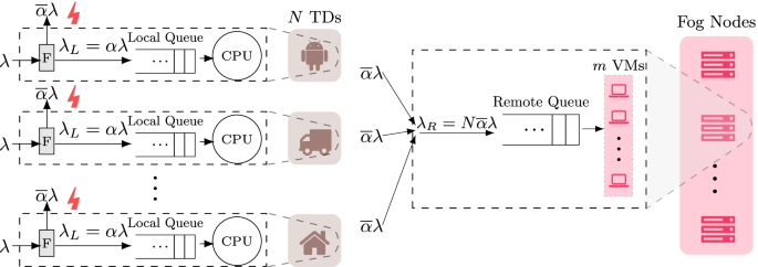

  

  Proposed queueing model. It comprises an M/G/1 queue at the TD and an M/G/m queue at the fog. The forwarder F offloads long tasks to the fog for remote processing, and retains short tasks at the TD for local processing

• 2. The fog node, serving the fog cell, has m VMs.

• 3. Each TD generates tasks according to a Poisson process with rate (parameter) λ. Consequently, if G denotes the task inter-generation time, then G is exponentially distributed, i.e. f_G(t)=λe^−λt, t≥0.

• 4. Each task requires a certain amount of time T if executed locally on the CPU of the TD. This time is assessed by the application that generates the task and is attached as a tag to the task (a meta-data field).

• 5. The task processing time T is a random variable (RV) of exponential distribution with parameter μ, i.e. f_T(t)=μe^−μt, t≥0.

• 6. Based on the value of T and a user defined threshold τ, a forwarding routine (F) at the TD forwards the task either to the local buffer, to be executed by the TD itself, or to the remote buffer at the fog, to be executed remotely by one of the m VMs there. In particular, if T<τ, the task is executed locally, and if T≥τ, it is executed remotely. In the present work, the former is called a local task and the latter is a remote task.

• 7. Via virtualization, each VM can be tailored to process a remote task in a certain amount of time. If this time is denoted by the RV S_R, then the service rate of the VM is $1/\mathbb {E}\left [ S_{R}\right ]$.

• 8. The local buffer size of each TD is infinite, and so is the remote buffer size at the fog. In modern times, memory units have become drastically inexpensive, encouraging the installation of gigantic buffers, which can be readily approximated as infinite with no loss of accuracy.

• 9. The task size in bytes is constant for all tasks. Consequently, for each task, the transmission time from the generating TD to the fog is also constant, and we will denote it by ξ.

• 10. Similarly, the task response size in bytes is constant for all tasks. Consequently, for each remote task response the transmission time from the fog to the TD that generated the task is also constant, and we will denote it by ψ.

Based on the forwarding threshold τ, and referring to Fig. 3, the fraction α of tasks that will be local is the area under the curve f_T(t)=μe^−μt from t=0 to t=τ. That is,

$$\begin{array}{*{20}l} \alpha &=\int_{0}^{\tau }f_{T}(u)du \\ &=\mu \int_{0}^{\tau }e^{-\mu u}du \\ &=1-e^{-\mu \tau} \end{array}$$

(1)

Fig. 3

The offloading threshold, τ, partitions the exponential curve into two truncated exponentials. Under the curve, the shaded area represents the fraction α of tasks that are local, while the complementary white area represents the fraction $\overline {\alpha }$ of tasks that are remote

Accordingly, $\overline {\alpha }=1-\alpha$ is the fraction of tasks that will be remote. We can also look at α as the probability that a generated task will be local, and $\overline {\alpha }=1-\alpha$ the probability that it will be remote. Accordingly, based on the splitting property of the Poisson process [39], the task arrival process at the local queue is Poisson with parameter

$$\lambda_{L}=\alpha \lambda$$

(2)

As the value of τ determines the amount of task offloading, it is a significant factor in determining the task response (TR) time. In turn, it has also a crucial impact on the TD energy consumption of the entire system. Specifically, lowering τ decreases CPU consumption, while it increases communications consumption, and vice versa.

Performance analysis

In this section, we will characterize the TR time at three different levels: local task, remote task, and task in general. Based on the assumptions in the preceding section, for a local task, the task service time is the same as its processing time. That is because, the task processing time is estimated based on the CPU of the TD where the task is generated. On the other hand, for a remote task, the two times are different, unless the fog is running the baseline virtualization mode with a unity speedup factor, k=1. We note also that although the task processing time is exponential at the time of generation, due to the forwarding process it is no longer exponential for both local and remote tasks. That is because the processing time for local tasks is upper bounded by τ, which represents a lower bound for remote tasks. Since the processing time needed by each task determines the service time of that task, whether locally or remotely, queueing models with general, rather than exponential (or Markovian) service times will be resorted to.

Local TR time

The local TR time will be the queueing time plus the service time at the local queueing system, which per the assumptions discussed above is an M/G/1 model [39]. The task service time S_L of this task will be exactly its task processing time, i.e. truncated exponential with parameter μ, upper bounded by τ. To find the distribution of S_L, consider for the moment an exponentially distributed RV A with parameter μ. The cumulative distribution of A given that A is upper bounded by some value τ is given by

$$\begin{array}{*{20}l} F_{A|A<\tau }(t) &=\mathbb{P}[A< t|A<\tau] \\ &=\frac{\mathbb{P}[A< t]}{\mathbb{P}[A < \tau]}, \end{array}$$

where t<τ. Since

$$\mathbb{P}[A< t]=\mu \int_{0}^{t}e^{-\mu x}dx=1-e^{-\mu t}\text{,}$$

(3)

then

$$F_{A|A<\tau }(t)=\frac{1-e^{-\mu t}}{1-e^{-\mu \tau}}.$$

Using this result, the distribution $f_{S_{L}}(t)$ of the service time S_L of a local task is given by

$$\begin{array}{*{20}l} f_{S_{L}}(t) &=\frac{d}{dx}F_{A|A<\tau }(t) \\ &=\frac{\mu e^{-\mu t}}{1-e^{-\mu \tau }}\text{.} \end{array}$$

(4)

With this distribution at hand, we can find the expectation $\mathbb {E}\left [ S_{L}\right ]$ of S_L as

$$\begin{array}{*{20}l} \mathbb{E}\left[ S_{L}\right] &=\int_{0}^{\tau }{tf}_{S_{L}}(t)dt \\ &=\frac{\mu }{1-e^{-\mu \tau }}\int_{0}^{\tau }te^{-\mu t}dt\text{.} \end{array}$$

Integrating by parts, we get

$$\mathbb{E}\left[ S_{L}\right] =\frac{1-e^{-\mu \tau }(1+\mu \tau)}{\mu \left(1-e^{-\mu \tau }\right) }\text{.}$$

(5)

In a similar manner, using integration by parts twice in the process, we can find the second moment of S_L to be

$$\begin{array}{*{20}l} \mathbb{E}\left[ S_{L}^{2}\right] &=\int_{0}^{\tau }t^{2}f_{S_{L}}(t)dt \\ &=\frac{\mu }{1-e^{-\mu \tau }}\int_{0}^{\tau }t^{2}e^{-\mu t}dt \\ &=\frac{2-\left(\mu^{2}\tau^{2}+2\mu \tau +2\right) e^{-\mu \tau }}{\mu^{2}\left(1-e^{-\mu \tau }\right)}. \end{array}$$

(6)

We are now in a position to find the expected TR time $\mathbb {E}\left [ R_{L}\right ]$ of a local task, which is the expected queueing time $\mathbb {E}\left [ Q_{L}\right ]$, i.e. the expected time spent at the local buffer before going to the local CPU, plus the expected service time $\mathbb {E}\left [ S_{L}\right ]$ at the local CPU. That is,

$$\mathbb{E}\left[ R_{L}\right] =\mathbb{E}\left[ Q_{L}\right] +\mathbb{E} \left[ S_{L}\right].$$

(7)

Based on the assumptions outlined above, the queueing model at the TD is an M/G/1 system, for which it can be shown [39] that

$$\mathbb{E}\left[ Q_{L}\right] =\frac{\lambda_{L}\mathbb{E}\left[ S_{L}^{2}\right]}{2\left(1-\lambda_{L}\mathbb{E}\left[ S_{L}\right] \right)}.$$

(8)

Using (7), (2), (5), (6), and (8), we can easily find the expected TR time of a local task to be

$$\mathbb{E}\left[ R_{L}\right] =\frac{\lambda \left(2-\left((1+\mu \tau)^{2}+1\right) e^{-\mu \tau }\right) }{2\mu \left(\mu -\lambda \left(1-e^{-\mu \tau}(1+\mu \tau)\right) \right) }+\frac{1-e^{-\mu \tau }(1+\mu\tau)}{\mu \left(1-e^{-\mu \tau }\right)}.$$

(9)

To validate this result, we will take its limit as τ→∞, which makes the fog inaccessible, getting

$$\begin{array}{*{20}l} {\lim}_{\tau \rightarrow \infty }\mathbb{E}\left[ R_{L}\right] &={\lim}_{\tau \rightarrow \infty }\left(\frac{\lambda \left(2-\left((1+\mu \tau)^{2}+1\right) e^{-\mu \tau }\right) }{2\mu \left(\mu -\lambda \left(1-e^{-\mu \tau }(1+\mu \tau)\right) \right) }\right) +{\lim}_{\tau\rightarrow \infty }\left(\frac{1-e^{-\mu \tau }(1+\mu \tau)}{\mu \left(1-e^{-\mu \tau }\right) }\right) \\ &=\frac{1}{\mu -\lambda}. \end{array}$$

(10)

This result is greatly reassuring, as it is the response (sojourn) time of an M/M/1 queueing system [39]. Indeed, without a fog all the TD generated tasks would go to the local queue which would then have exponential inter-arrival time (with parameter λ) and exponential service time (with parameter μ), both being the defining characteristics of an M/M/1 queueing system.

The stability of the local queueing system is ensured by keeping its arrival rate strictly less than its service rate, or $\lambda _{L}<1/\mathbb {E}\left [ S_{L}\right ]$, which is equivalent to the task generation rate λ satisfying

$$\lambda <\frac{\mu }{1-e^{-\mu \tau }(1+\mu \tau)}.$$

(11)

Remote TR time

At each TD, a fraction $\overline {\alpha }=e^{-\mu \tau }$ of the Poisson stream of tasks generated is offloaded to the fog for remote execution. Based on the splitting (thinning) property of Poisson processes [40], a Poission stream with parameter $\overline {\alpha }\lambda$ arrives at the fog from each TD. Thus, N Poisson streams arrive at the fog from the N TDs of the cell. Based on the merging (superposition) property of Poisson processes [40], the arrival process at the remote queue is Possion with parameter

$$\lambda_{R}=N\overline{\alpha }\lambda =N\lambda e^{-\mu \tau }$$

(12)

The expected remote TR time is the sum of the expected remote queueing time, expected remote service time, and both the transmission time ξ of the task from the TD to the fog, and the transmission time ψ of the task’s response from the fog back to the TD. Let R_R, Q_R and S_R be the TR time, task queueing time and task service time, respectively, at the fog. Accordingly, the expected TR time $\mathbb {E}\left [ R_{R}\right ]$ is given by

$$\mathbb{E}\left[ R_{R}\right] =\mathbb{E}\left[ Q_{R}\right] +\mathbb{E} \left[ S_{R}\right] +\xi +\psi \text{.}$$

(13)

Since the arrival process at the fog is Poisson, and since the processing time is not exponential, but rather a truncated exponential, then the remote queueing system at the fog is a perfect M/G/m system [39]. To evaluate the expected queueing time at the fog there is a very good approximation [41]

$$\mathbb{E}\left[ Q_{R}\right] \approx \frac{\lambda_{R}^{m}\mathbb{E}\left[ S_{R}^{2}\right] \left(\mathbb{E}\left[ S_{R}\right] \right)^{m-1}}{2\left(m-1\right) !\left(m-\lambda_{R}\mathbb{E}\left[ S_{R}\right]\right)^{2}\digamma },$$

(14)

where $\digamma$ is given by

$$\digamma =\sum_{i=0}^{m-1}\frac{\left(\lambda_{R}\mathbb{E}\left[ S_{R}\right] \right)^{i}}{i!}+\frac{\left(\lambda_{R}\mathbb{E}\left[ S_{R}\right] \right)^{m}}{\left(m-1\right) !\left(m-\lambda_{R}\mathbb{E}\left[ S_{R}\right] \right) }\text{,}$$

with $\mathbb {E}\left [ S_{R}\right ]$ and $\mathbb {E}\left [ S_{R}^{2}\right ]$ being the first moment (expectation) and the second moment, respectively, of the remote task service time S_R. Incidentally, this approximation is so good that it yields, if we substitute in it m=1, the exact expression (5) of the M/G/1 system.

The stability of the remote queueing system is ensured by making its arrival rate strictly less than its service rate, i.e.

$$\lambda_{R}<\frac{m}{\mathbb{E}[S_{R}]}.$$

(15)

Next, we will consider three modes for the remote TR time, corresponding to three virtualization modes. For each mode, the task service time will be different due to the change in the virtualization mode. The change will be reflected in the two moments $\mathbb {E}\left [ S_{R}\right ]$ and $\mathbb {E}\left [ S_{R}^{2}\right ]$ needed in Eq. (14).

Perfect virtualization (constant service time):

In the perfect virtualization mode, the fog will place for each incoming task a VM with computational power exactly proportional to the computational needs of the arriving task. For example, if a task is computationally heavy, the fog will place for it an equally computationally heavy VM and if it is computationally light, the fog will place for it an equally computationally light VM, such that the task service time is always a constant c>0. Consequently, the queueing model at the fog for this mode is of an M/D/m system.

Let $R_{R_{P}}$, $Q_{R_{P}}$ and $S_{R_{P}}$ be the TR time, queueing time and service time, respectively, of remote tasks under the perfect virtualization mode. Given the fact that $S_{R_{P}}$ is a degenerate RV of value c, then the queueing model at the fog for this mode is an M/D/m system, with the first two moments of $S_{R_{P}}$ being

$$\mathbb{E}\left[ S_{R_{P}}\right]=c$$

(16)

and

$$\mathbb{E}\left[ S_{R_{P}}^{2}\right] =c^{2}.$$

(17)

Using (13), (14), (16), (17), and (12), we can find the expected TR time in the perfect virtualization mode to be

$$\mathbb{E}\left[ R_{R_{P}}\right] \approx \frac{\lambda_{R}^{m}c^{m+1}}{2\left(m-1\right)!\left(m-\lambda_{R}c\right)^{2}\digamma_{R_{P}}}+c+\xi +\psi \text{,}$$

(18)

where

$$\digamma_{R_{P}}=\sum\limits_{i=0}^{m-1}\frac{\left(\lambda_{R}c\right)^{i}}{i!}+\frac{\left(\lambda_{R}c\right)^{m}}{\left(m-1\right) !\left(m-\lambda_{R}c\right)}.$$

Using (15), the stability condition of the remote queueing system for the perfect virtualization mode is

$$\lambda_{R}<\frac{m}{c}.$$

Semiperfect virtualization (uniform service time):

The semiperfect virtualization mode is more flexible than the perfect virtualization mode. Here, the fog cannot guarantee all arriving tasks the same service time, as was the case in the perfect virtualization mode. Rather, it guarantees service times that are uniformly distributed between pre-defined limits a and b, with a<b. Any remote task, no matter how heavy or how light will be served by a VM at the fog within these two limits, with any value between the two limits being equally likely.

Let $R_{R_{S}}$, $Q_{R_{S}}$ and $S_{R_{S}}$ be the TR time, queueing time and service time, respectively, of remote tasks under the semiperfect virtualization mode. Given the fact that $S_{R_{S}}$ is uniformly distributed, $S_{R_{S}}\sim {U}[a,b]$, then the queueing model at the fog for this mode is an M/U/m system, with the first two moments of $S_{R_{S}}$ being

$$\mathbb{E}[S_{R_{S}}]=\frac{a+b}{2},$$

(19)

and

$$\mathbb{E}[S_{R_{S}}^{2}]=\frac{b^{2}+ab+a^{2}}{3}.$$

(20)

Using (13), (14), (19), (20), and (12), we can find the expected TR time in the perfect virtualization mode to be

$$\mathbb{E}\left[ R_{R_{S}}\right] \approx \frac{\lambda_{R}^{m}\frac{b^{2}+ab+a^{2}}{3}\left(\frac{a+b}{2}\right)^{m-1}}{2\left(m-1\right) !\left(m-\lambda_{R}\frac{a+b}{2}\right)^{2}\digamma_{R_{S}}}+\frac{a+b}{2}+\xi +\psi,$$

(21)

where

$$\digamma_{R_{S}}=\sum\limits_{i=0}^{m-1}\frac{\left(\lambda_{R}\frac{a+b}{2}\right)^{i}}{i!}+\frac{\left(\lambda_{R}\frac{a+b}{2}\right)^{m}}{\left(m-1\right) !\left(m-\lambda_{R}\frac{a+b}{2}\right)}.$$

Using (15), the stability condition of the remote queueing system for the semiperfect virtualization mode is

$$\lambda_{R}<\frac{2m}{a+b}.$$

Baseline virtualization (truncated exponential service time):

Unlike the above two modes, which are novel, this mode is the default in the literature. In this mode, the arriving tasks are served at the fog by midentical VMs, each having the same computational power. That is, the computational power of a VM is the same as any other VM in the fog, and generally is k≥1 times the computational power of a TD. In other words, the computational power of any VM is not related to the computational needs of the arriving task. The computational needs of a remote task are related to the processing time of that task, where the latter is a truncated exponential time with parameter μ and is lower bounded by some value τ>0, as shown in Fig. 3.

Let $R_{R_{B}}$, $Q_{R_{B}}$ and $S_{R_{B}}$ be the TR time, queueing time and service time, respectively, of remote tasks under the baseline virtualization mode. Given the fact that $S_{R_{B}}$ is generally distributed, then the queueing model at the fog for this mode is of the M/G/m system, and the first two moments of $S_{R_{B}}$ will be obtained next.

Before computing the moments, consider for a moment an exponential RV A with parameter μ and lower bounded by a positive value τ. Then for t≥τ, we have the conditional cumulative distribution

$$\begin{array}{*{20}l} F_{A|A\geq \tau }(t) &=\mathbb{P}[A< t|A\geq \tau ] \\ &=\frac{e^{-\mu \tau }-e^{-\mu t}}{e^{-\mu \tau }} \end{array}$$

This result can be used to find the conditional distribution

$$\begin{array}{*{20}l} f_{A|A\geq \tau }(t) &=\frac{d}{dt}F_{A|A\geq \tau }(t) \\ &=\frac{\mu e^{-\mu t}}{e^{-\mu \tau }},\qquad t\geq \tau \text{.} \end{array}$$

(22)

Re-scaling the distribution to account for the VM speedup factor k, gives the distribution of the task service time

$$f_{S_{R_{B}}}(t)=\frac{k\mu e^{-k\mu t}}{e^{-\mu \tau }},\qquad t\geq \frac{\tau }{k}.$$

(23)

This result can be validated by integrating from $\frac {\tau }{k}$ to ∞ to obtain 1.

Now that we have the distribution $f_{S_{R_{B}}}(t)$ at hand, the first moment of $S_{R_{B}}$ is

$$\begin{array}{*{20}l} \mathbb{E}\left[ S_{R_{B}}\right] &=\int_{\frac{\tau }{k}}^{\infty}{tf}_{S_{R_{B}}}(t)dt \\ &=\frac{k\mu}{e^{-\mu \tau}}\int_{\frac{\tau }{k}}^{\infty }te^{-k\mu t}dt \end{array}$$

Using integration by parts, we get

$$\mathbb{E}\left[ S_{R_{B}}\right] =\frac{k\mu }{e^{-\mu \tau }}\left[ \frac{e^{-\mu \tau }}{k^{2}\mu }\left(\tau +\frac{1}{\mu }\right) \right] =\frac{1}{k}\left(\tau +\frac{1}{\mu }\right) =\frac{\tau \mu +1}{k\mu }$$

(24)

This result is logical, since without the speedup factor the expectation of a truncated exponential would be $\mathbb {E}\left [ S_{R}\right ] =\tau +\frac {1}{\mu }$.

In a similar manner, utilizing integration by parts twice in the process, the second moment of $S_{R_{B}}$ is

$$\begin{array}{*{20}l} \mathbb{E}\left[ S_{R_{B}}^{2}\right] &=\int_{\frac{\tau }{k}}^{\infty}t^{2}f_{S_{R}}(t)dt \\ &=\frac{k\mu }{e^{-\mu \tau }}\int_{\frac{\tau }{k}}^{\infty }t^{2}e^{-k\mu t}dt \\ &=\frac{\left(\mu \tau \right)^{2}+2\mu \tau +2}{\left(k\mu \right)^{2}} \end{array}$$

(25)

Using (13), (14), (24), (25), and (12), we can find the expected TR time in the baseline virtualization mode to be

$$\mathbb{E}\left[ R_{R_{B}}\right] \approx \frac{\lambda_{R}^{m}\frac{\left(\mu \tau \right)^{2}+2\mu \tau +2}{\left(k\mu \right)^{2}}\left(\frac{\tau \mu +1}{k\mu }\right)^{m-1}}{2\left(m-1\right) !\left(m-\lambda_{R}\frac{\tau \mu +1}{k\mu }\right)^{2}\digamma_{R_{B}}}+\frac{\tau \mu +1}{k\mu }+\xi +\psi,$$

(26)

where

$$\digamma_{R_{B}}=\sum\limits_{i=0}^{m-1}\frac{\left(\lambda_{R}\frac{\tau \mu +1}{k\mu }\right)^{i}}{i!}+\frac{\left(\lambda_{R}\frac{\tau \mu +1}{k\mu }\right)^{m}}{\left(m-1\right) !\left(m-\lambda_{R}\frac{\tau \mu +1}{k\mu }\right)}.$$

Using (15), the stability condition of the remote queueing system for the baseline virtualization mode is

$$\lambda_{R}<\frac{km\mu }{\tau \mu +1}.$$

Overall TR time

Above we have calculated the expected TR time for both local and remote tasks. However, since task offloading is an internal activity, the metric that the end user cares about is the overall TR time, which is the time between the instant a task is generated by an application at the TD and the instant the response of that task is received back by the application. Indeed, the end user does not, and should not, care much about whether the task was executed locally or remotely. What the end user cares about is the overall TR time defined next.

Definition 1

(Overall TR time): The overall TR time, R_O, is the amount of time between the instant a task is generated by an application at the TD and the instant the response of that task is received back by the application, regardless of whether the task was served locally or remotely.

From Definition 1, it is clear that the expected overall TR time $\mathbb {E}\left [ R_{O}\right ]$ is the weighted sum of the expected local and remote TR times. That is,

$$\mathbb{E}\left[ R_{O}\right] =\alpha \mathbb{E}\left[ R_{L}\right] + \overline{\alpha }\mathbb{E}\left[ R_{R}\right],$$

(27)

Using this formula and Eq. (9), we can generate three equations for the overall TR times corresponding to the three modes above: perfect, semiperfect and baseline virtualization.

Perfect virtualization (constant service time):

Using (27), the expected overall TR time, $\mathbb {E}\left [ R_{O_{P}}\right ]$, for the perfect virtualization mode is given by

$$\mathbb{E}\left[ R_{O_{P}}\right] =\alpha \mathbb{E}\left[ R_{L}\right] +\overline{\alpha }\mathbb{E}\left[ R_{R_{P}}\right],$$

(28)

where α is given by (1), $\mathbb {E}\left [ R_{L}\right ]$ by (9), and $\mathbb {E}\left [ R_{R_{P}}\right ]$ by (18).

Semiperfect virtualization (uniform service time):

Using (27), the expected overall TR time, $\mathbb {E}\left [ R_{O_{S}}\right ]$, for the semiperfect virtualization mode is given by

$$\mathbb{E}\left[ R_{O_{S}}\right] =\alpha \mathbb{E}\left[ R_{L}\right] +\overline{\alpha }\mathbb{E}\left[ R_{R_{S}}\right],$$

(29)

where α is given by (1), $\mathbb {E}\left [ R_{L}\right ]$ by (9), and $\mathbb {E}\left [ R_{R_{S}}\right ]$ by (21).

Baseline virtualization (truncated exponential service time):

Using (27), the expected overall TR time, $\mathbb {E}\left [ R_{O_{B}}\right ]$, for the baseline virtualization mode is given by

$$\mathbb{E}\left[ R_{O_{B}}\right] =\alpha \mathbb{E}\left[ R_{L}\right] +\overline{\alpha }\mathbb{E}\left[ R_{R_{B}}\right],$$

(30)

where α is given by (1), $\mathbb {E}\left [ R_{L}\right ]$ by (9), and $\mathbb {E}\left [ R_{R_{B}}\right ]$ by (26).

Numerical results

The aim of this section is two fold. First, we will validate the analytical results obtained in the preceding section using simulation. To this end, we have developed a discrete event Monte Carlo simulation program to compute the TR time for each of the three virtualization modes considered. The program is written in Python (We have made the code publicly available at https://github.com/Virtualization-Fog/FogV.git). It was run on a PC having an Intel i7 processor @ 2.4 GHz, with 16 GB of main memory. Each simulation experiment comprised 4 million runs, which were found enough to reach convergence.

The second aim of this section is to investigate the impact of system parameters on the TR time. To this end, numerous fog examples have been assumed. For each example, the TR time has been calculated for different sets of parameters twice, once using the equations obtained in the preceding section and once using the simulation program. As will be seen in the figures below, the match between the analytical results and the simulation results is quite spectacular.

All the factors that impact the TR time were incorporated in the experiments. Seven of these factors that are common in all modes are shown in Table 2. Besides these seven factors, there are four that are mode specific: c in the perfect mode, a and b in the semiperfect mode, and k in the baseline mode. In all the experiments, we fixed the task transmission time from a TD to the fog at ξ=20 sec, and the response transmission time form the fog to the TD at ψ=10 sec. This means that we implicitly assume that the task size in bytes is twice as large as the response size. Furthermore, we fixed the expected task processing time at 909 sec, or μ=1/909=0.0011 task/sec. Recall that the processing time of a task is estimated at the computational power of the TD.

Table 2 Main system parameters

For each of the three considered modes, we carried out four experiments, each designed to validate an analytical result on the one hand, and assess the impact of some parameter on the TR time on the other hand. For each of these four experiments, we end up displaying three types of curves: one for the expected local TR time, one for the expected remote TR time, and one for the overall TR time. Each type has two curves, one from the simulation experiment and one from the corresponding analytical equation. As the Figures below illustrate, for all three modes, the expected local TR time is substantially larger than the expected remote TR time. This confirms the feasibility of using a fog in general and the proposed virtualization modes in particular. It can also be seen that in each mode the expected overall TR time curve, which is what the end user cares about, falls between the local and remote curves as anticipated.

At the end of this section, we provide a Figure comparing the overall TR time for all three modes. The Figure shows vividly that proper virtualization, either perfectly or semiperfectly, is more fruitful for TR time reduction than using VMs each of them nineteen times faster than a TD.

Remote TR time under perfect virtualization

The perfect virtualization mode is characterized by having a constant service time c at the fog all remote tasks. In this section, we use c=40 sec in all four experiments pertaining to this mode. The analytical and simulation results for this mode are displayed in Fig. 4. The analytical results are obtained from Eqs. (18), (9) and (28), which provide the expected remote TR time $\mathbb {E}[R_{R_{P}}]$, expected local TR time $\mathbb {E}[R_{L}]$, and expected overall TR time $\mathbb {E}[R_{O_{P}}]$, respectively, for the semiperfect virtualization mode. The simulation results are obtained from running our simulator 4 million runs.

Fig. 4

TR time for perfect virtualization mode, where μ=0.0011 task/sec, α=0.63, c=40 sec, ξ=20 sec, and ψ=10 sec. a TR time versus the task inter-generation λ. b TR time versus the off-loading threshold τ. c TR time versus the number of TDs N. d TR time versus the number of VMs m

First, Fig. 4a displays the impact of the task generation rate λ on the TR time. The system parameters are fixed at N=500 TDs, m=5 VMs, and τ=900 sec. As can be seen in the Figure, the TR time, for all three curves, increases almost linearly with λ until just before the instability point at the end of the λ range. To understand this curve behavior, recall that the TR time is made up of three components: queueing time, service time and round trip transmission time. For the perfect mode, the last two components are constant. It is only the first component that increases with λ, slightly and linearly at the beginning then heavily and non-linearly as the queueing system at the fog approaches its instability point (at the end of the curve). Second, Fig. 4b displays the impact of the task off-loading threshold τ on the expected TR time. The system parameters are fixed at N=500 TDs, m=5 VMs, and λ=0.0001 task/sec. As can be seen in the Figure, the remote TR time is roughly a straight line. That is because every task, regardless of its computational needs, is completed in exactly the same time, 40 sec. On the other hand, as τ increases, more tasks are processed locally, resulting in a longer local TR time. It is only the local TR time that increases with τ non-linearly, since the service times of local tasks are exponentially distributed. Third, Fig. 4c displays the impact of the number N of TDs in the fog cell on the TR time. The system parameters are fixed at τ=900 sec, m=5 VMs, and λ=0.0001 task/sec. From this Figure we note that the local TR time does not change over the range of N. This is intuitive because processing in each TD is independent of other TDs in the cell. When N is high (in our experiment, N>1500), the remote TR time, on the other hand, increases significantly since much traffic pours into the fog, increasing the queueing time there somewhat. Finally, Fig. 4d displays the impact of the number m of VMs in the fog node on the expected TR time. The system parameters are fixed at τ=900 sec, N=500 VMs, and λ=0.0001 task/sec. This Figure has two observations. First, changing the number m of VMs has no influence on the local TR time $\mathbb {E}\left [ R_{L}\right ]$, which is intuitive. Second, the impact of m on the remote TR time, $\mathbb {E}\left [ R_{R_{P}}\right ]$, is almost unchanged after a small value of m, here after m=5. That is because as m increases the queueing time in the fog decreases, at some point becoming negligible compared to the other two constant components of the TR time: round trip transmission time and service time.

Remote TR time under semiperfect virtualization

The semiperfect virtualization mode is characterized by having a uniformly distributed service time, with parameters a and b, where a<b, for all remote tasks. We fixed a=30 sec and b=100 sec in all four experiments pertaining to this mode. The analytical and simulation results for this mode are displayed in Fig. 5. The analytical results are obtained from Eqs. (21), (9) and (29), which provide the expected remote TR time $\mathbb {E}[R_{R_{S}}]$, expected local TR time $\mathbb {E}[R_{L}]$, and expected overall TR time $\mathbb {E}[R_{O_{S}}]$, respectively, for the perfect virtualization mode. The simulation results are obtained from running our simulator 4 million runs. We can notice that the behavior of the curves of this Figure is very close to that of the curves of the preceding one, Fig. 4. That is because the processing time now is confined uniformly in the interval [30,100]. Therefore, we will not repeat below the detailed comments given above for the perfect mode.

Fig. 5

TR time for the semiperfect virtualization mode, where μ=0.0011 task/sec, α=0.63, a=30, b=100, ξ=20 sec. a TR time versus the task inter-generation λ. b TR time versus the off-loading threshold τ. c TR time versus the number of TDs N. d TR time versus the number of VMs m

Figure 5a displays the impact of the task generation rate λ on the expected TR time. The system parameters for this experiment are fixed at N=500 TDs, m=5 VMs, μ=0.0011 task/sec, and τ=900 sec. Figure 5b displays the impact of the task off-loading threshold τ on the expected TR time. The system parameters for this experiment are fixed at N=500 TDs, m=5 VMs, μ=0.0011 task/sec, and λ=0.0001 task/sec. Figure 5c displays the impact of the number N of TDs in the fog cell on the expected TR time. The system parameters for this experiment are fixed at τ=900 sec, m=5 VMs, μ=0.0011 task/sec, and λ=0.0001 task/sec. Figure 5d displays the impact of the number m of VMs in the fog node on the expected TR time. The system parameters for this experiment are fixed at τ=900 sec, N=500 VMs, μ=0.0011 task/sec, and λ=0.0001 task/sec.

Remote TR time under baseline virtualization

The baseline virtualization mode is characterized by having a truncated exponential service time for all remote tasks, with a speedup factor k. We fixed k=19 in all four experiments pertaining to this mode. The analytical and simulation results for this mode are displayed in Fig. 4. Note that the speedup factor k impacts only the remote TR time. As k increases, the remote TR time decreases, and vice versa. The analytical and simulation results for this mode are displayed in Fig. 6, where we can see that the match between both is remarkable. The analytical results are obtained from Eqs. (26), (9) and (30), which provide the expected remote TR time $\mathbb {E}[R_{R_{B}}]$, expected local TR time $\mathbb {E}[R_{L}]$, and expected overall TR time $\mathbb {E}[R_{O_{B}}]$, respectively, for the baseline virtualization mode. The simulation results are obtained from running our simulator 4 million runs.

Fig. 6

TR time for the baseline mode, where μ=0.0011 task/sec, α=0.63, k=19, ξ=20 sec, and ψ=10 sec. a TR time versus the task inter-generation λ. b TR time versus the off-loading threshold τ. c TR time versus the number of TDs N. d Response times versus the number of VMs m

Figure 6a displays the impact of the task generation rate λ on the expected TR time. The system parameters for this experiment are fixed at N=500 TDs, m=5 VMs, and τ=900 sec. From this Figure draw the following two points. First, the local TR time is largely linear, increasing with λ very slightly. This is to be expected since the local queueing system is of the M/G/1 type. Second, the remote TR time is almost linear at the beginning, increasing slightly with λ till some point, roughly λ=0.0028, where it increases dramatically. This is also intuitive as when λ reaches that dramatic point it produces, in light of the large number of TDs, N=500, huge traffic into the fog, jacking up queueing time there drastically. Figure 6b displays the impact of the task off-loading threshold τ on the expected TR time. The system parameters for this experiment are fixed at N=500 TDs, m=5 VMs, and λ=0.0001 task/sec. It is interesting to note that the higher the τ, the higher both the local TR time and remote TR time, which is justified as follows. First, as τ increases more tasks with potentially long service times (potentially as long as τ) are retained for local processing, which increases the local TR time. Second, as τ increases it is true that the number of tasks offloaded to the fog will be less, but their service times will be large, specifically larger than τ. Figure 6c displays the impact of the number N of TDs in the fog cell on the expected TR time. The system parameters for this experiment are τ=900 sec, m=5 VMs, and λ=0.0001 task/sec. We first note that the local TR time is independent of N which is intuitive since each TD operates independently of all the TDs of the fog cell no matter what their number is. We also note that the remote TR time exceeds the local TR time over the range of N until some value, roughly N =130 TDs. That is because the fog receives traffic from the N TDs, so the higher the N the higher the remote TR time. This problem was not seen by the way in the other two modes, which confirms their superiority over the baseline mode. Finally, Fig. 6d displays the impact of the number m of VMs in the fog node on the expected TR time. The system parameters for this experiment are fixed at τ=900 sec, N=500 VMs, and λ=0.0001 task/sec. The Figure illustrates, like in the other two modes, that increasing the number m of VMs after some minimum, here m=4, is pointless.

Comparison of overall TR time under all three virtualization modes

Now it is time to compare the overall TR time in all three modes. We plot in Fig. 7 the expected overall TR times: $\mathbb {E}[R_{O_{P}}]$ given by (28), $\mathbb {E}[R_{O_{S}}]$ given by (29) and $\mathbb {E}[R_{O_{B}}]$ given by (30). The other parameters here have the values: μ=0.0011 task/sec, α=0.63, k=19, ξ=20 sec, ψ=10 sec, a=30, b=100, and c=40 sec. Plotted also are the simulation results which match the analytical results spectacularly.

Fig. 7

Comparison of the overall TR times for perfect, semiperfect and baseline modes, $\mathbb {E}[R_{O_{P}}]$ represented in (28), $\mathbb {E}[R_{O_{S}}]$ represented in (29) and $\mathbb {E}[R_{O_{B}}]$ represented in (30) where μ=0.0011 task/sec, α=0.63, k=19, ξ=20 sec, ψ=10 sec, a=30, b=100, and c=40 sec

Figure 7a displays the impact of the task generation rate λ on the expected TR time. The system parameters for this graph are fixed at N=500 TDs, m=5 VMs, μ=0.0011 task/sec, and τ=900 sec. Figure 7b displays the impact of the task off-loading threshold τ on the expected TR time. The system parameters for this graph are fixed at N=500 TDs, m=5 VMs, μ=0.0011 task/sec, and λ=0.0001 task/sec. Figure 7c displays the impact of the number N of TDs in the fog cell on the expected TR time. The system parameters for this graph are fixed at τ=900 sec, m=5 VMs, μ=0.0011 task/sec, and λ=0.0001 task/sec. Figure 7d displays the impact of the number m of VMs in the fog node on the expected TR time. The system parameters for this graph are fixed at τ=900 sec, N=500 VMs, μ=0.0011 task/sec, and λ=0.0001 task/sec. As all four graphs show, using virtualization either perfectly or semiperfectly gives rise to substantial improvement in the overall TR time.

Conclusions

In this article we have presented a novel study to characterize the TR time in a fog enabled IoT network under three different virtualization modes, departing from previous studies, which have focused on such traditional fog issues as scheduling, load balancing and live migration. The main mathematical tool used in our work is queueing theory, which lends itself elegantly to the task waiting phenomenon, either locally at the TD or remotely at the fog. Two queueing models in particular have been principally considered, the M/G/1 and M/G/m. To validate the analytical results obtained by queueing theory, we have developed simulation software, in the Python language, applying Monte Carlo and discrete event notions. The experimental work shows clearly that the match between the analytical and simulation results is excellent.

The main conclusion of this study is that virtualization can be used favorably to reduce TR time. In particular, the perfect mode is the best in this regard. However, is admittedly hard to implement practically. Therefore, the semiperfect mode comes in as a viable alternative, as it is easy to implement while it can reduce the TR time significantly in comparison with the baseline mode.

Directions where our work can be extended in the future include repeating the study with variable transmission times, from the TD to the fog and from the fog to the TD, using reasonable distributions. They also include considering mobile TDs, i.e. TDs that move across different cells, rather than just within a single cell.

References

Khan AUR, Othman M, Madani SA, Ullah KS (2014) A survey of mobile cloud computing application models. IEEE Commun Surv Tutor 16(1):393–413. https://doi.org/10.1109/SURV.2013.062613.00160.
Sanaei Z, Abolfazli S, Gani A, Buyya R (2014) Heterogeneity in mobile cloud computing: Taxonomy and open challenges. IEEE Commun Surv Tutor 16(1):369–392. https://doi.org/10.1109/SURV.2013.050113.00090.
Ray B (2019) The Role of Cloud Computing and Fog Computing in IoT. https://www.iotforall.com/cloud-fog-computing-iot. Accessed 24 Oct 2021.
Marinescu DC (2018) Cloud Computing - Theory and Practice, Second Edition. Elsevier, San Francisco.
Hanes D, Salgueiro G, Grossetete P, Barton R, Henry J (2017) IoT Fundamentals: Networking Technologies, Protocols, and Use Cases for the Internet of Things, First Edition. Cisco Press, Indianapolis.
Tadakamalla U, Menascé Daniel A (2018) Fogqn: An analytic model for fog/cloud computing In: 2018 IEEE/ACM International Conference on Utility and Cloud Computing Companion, UCC Companion 2018, Zurich, Switzerland, December 17-20, 2018, 307–313.. IEEE. https://doi.org/10.1109/UCC-Companion.2018.00073.
Abdelradi YM, El-Sherif AA, Afify LH (2021) A queueing theory approach to traffic offloading in heterogeneous cellular networks. AEU Int J Electron Commun 139:153910. https://doi.org/10.1016/j.aeue.2021.153910.
Abdul Majeed A, Kilpatrick P, Spence ITA, Varghese B (2020) Modelling fog offloading performance In: 4th IEEE International Conference on Fog and Edge Computing, ICFEC 2020, Melbourne, Australia, May 11-14, 2020, 29–38.. IEEE. https://doi.org/10.1109/ICFEC50348.2020.00011.
Rista A, Ajdari J, Zenuni X (2020) Cloud computing virtualization: A comprehensive survey In: 43rd International Convention on Information, Communication and Electronic Technology, MIPRO 2020, Opatija, Croatia, September 28 - October 2, 2020, 462–472.. IEEE. https://doi.org/10.23919/MIPRO48935.2020.9245124.
Chaudhari S, Mani RS, Raundale P (2016) Sdn network virtualization survey In: 2016 International Conference on Wireless Communications, Signal Processing and Networking (WiSPNET), 650–655. https://doi.org/10.1109/WiSPNET.2016.7566213.
Mahmud MR, Afrin M, Razzaque MA, Hassan MM, Alelaiwi A, AlRubaian MA (2016) Maximizing quality of experience through context-aware mobile application scheduling in cloudlet infrastructure. Softw Pract Exp 46(11):1525–1545. https://doi.org/10.1002/spe.2392.
Bahl P, Han RY, Li E, Satyanarayanan M (2012) Advancing the state of mobile cloud computing In: The Third ACM Workshop on Mobile Cloud Computing and Services, ACM, 21–28. https://doi.org/10.1145/2307849.2307856.
Al-Fuqaha AI, Guizani M, Mohammadi M, Aledhari M, Ayyash M (2015) Internet of things: A survey on enabling technologies, protocols, and applications. IEEE Commun Surv Tutorials 17(4):2347–2376. https://doi.org/10.1109/COMST.2015.2444095.
Usmani Z, Singh S (2016) A survey of virtual machine placement techniques in a cloud data center. Procedia Comput Sci 78:491–498. https://doi.org/10.1016/j.procs.2016.02.093.
Feng D, Wu Z, Zuo D, Zhang Z (2019) Erp: An elastic resource provisioning approach for cloud applications. PLoS ONE 14:0216067. https://doi.org/10.1371/journal.pone.0216067.
Fourati M, Marzouk S, Jmaiel M (2022) Epma: Elastic platform for microservices-based applications: Towards optimal resource elasticity. J Grid Comput 20. https://doi.org/10.1007/s10723-021-09597-5.
Virtual Machine Desired State Configuration. https://flings.vmware.com/virtual-machine-desired-state-configuration. Accessed 22 Jul 2022.
Nottingham C (2021) Change the size of a virtual machine. https://docs.microsoft.com/en-us/azure/virtual-machines/resize-vm?tabs=portal. Accessed 13 Mar 2022.
Saeik F, Avgeris M, Spatharakis D, Santi N, Dechouniotis D, Violos J, Leivadeas A, Athanasopoulos N, Mitton N, Papavassiliou S (2021) Task offloading in edge and cloud computing: A survey on mathematical, artificial intelligence and control theory solutions. Comput Netw 195:108177. https://doi.org/10.1016/j.comnet.2021.108177.
Ushakova M, Ushakov Y, Bolodurina I, Shukhman A, Legashev L, Parfenov D (2021) Creation of adequate simulation models to analyze performance parameters of a virtual fog computing infrastructure. Procedia Comput Sci 186:603–610. https://doi.org/10.1016/j.procs.2021.04.182.
Wu H, Wolter K (2018) Stochastic analysis of delayed mobile offloading in heterogeneous networks. IEEE Trans Mob Comput 17(2):461–474. https://doi.org/10.1109/TMC.2017.2711014.
Aljanabi S, Chalechale A (2021) Improving iot services using a hybrid fog-cloud offloading. IEEE Access 9:13775–13788. https://doi.org/10.1109/ACCESS.2021.3052458.
Shahhosseini S, Anzanpour A, Azimi I, Labbaf S, Seo D, Lim S-S, Liljeberg P, Dutt N, Rahmani AM (2021) Exploring computation offloading in iot systems. Inf Syst:101860. https://doi.org/10.1016/j.is.2021.101860.
Jaddoa A, Sakellari G, Panaousis E, Loukas G, Sarigiannidis PG (2020) Dynamic decision support for resource offloading in heterogeneous internet of things environments. Simul Model Pract Theory 101:102019. https://doi.org/10.1016/j.simpat.2019.102019.
Sun C, Zhou J, Liuliang J, Zhang J, Zhang X, Wang W (2018) Computation offloading with virtual resources management in mobile edge networks In: 87th IEEE Vehicular Technology Conference, VTC Spring 2018, Porto, Portugal, June 3-6, 2018, 1–5.. IEEE. https://doi.org/10.1109/VTCSpring.2018.8417681.
Rekha PM, Dakshayini M (2018) Dynamic cost-load aware service broker load balancing in virtualization environment. Procedia Comput Sci 132:744–751. https://doi.org/10.1016/j.procs.2018.05.086.
Maiti P, Sahoo B, Turuk AK, Kumar A, Choi BJ (2021) Internet of things applications placement to minimize latency in multi-tier fog computing framework. ICT Express. https://doi.org/10.1016/j.icte.2021.06.004.
Chebaane A, Spornraft S, Khelil A (2020) Container-based task offloading for time-critical fog computing In: 3rd IEEE 5G World Forum, 5GWF 2020, Bangalore, India, September 10-12, 2020, 205–211.. IEEE. https://doi.org/10.1109/5GWF49715.2020.9221486.
Hwang J, Nkenyereye L, Sung N, Kim J, Song J (2021) Iot service slicing and task offloading for edge computing. IEEE Internet Things J 8(14):11526–11547. https://doi.org/10.1109/JIOT.2021.3052498.
Hejja K, Berri S, Labiod H (2021) Network slicing with load-balancing for task offloading in vehicular edge computing. Veh Commun:100419. https://doi.org/10.1016/j.vehcom.2021.100419.
Li J, Jin J, Yuan D, Zhang H (2018) Virtual fog: A virtualization enabled fog computing framework for internet of things. IEEE Internet Things J 5(1):121–131. https://doi.org/10.1109/JIOT.2017.2774286.
Li J, Liang W, Ma Y (2021) Robust service provisioning with service function chain requirements in mobile edge computing. IEEE Trans Netw Serv Manag 18(2):2138–2153. https://doi.org/10.1109/TNSM.2021.3062650.
Zhang Q, Gui L, Hou F, Chen J, Zhu S, Tian F (2020) Dynamic task offloading and resource allocation for mobile-edge computing in dense cloud RAN. IEEE Internet Things J 7(4):3282–3299. https://doi.org/10.1109/JIOT.2020.2967502.
Cao K, Li L, Cui Y, Wei T, Hu S (2021) Exploring placement of heterogeneous edge servers for response time minimization in mobile edge-cloud computing. IEEE Trans Ind Inf 17(1):494–503. https://doi.org/10.1109/TII.2020.2975897.
Sopin ES, Daraseliya AV, Correia LM (2018) Performance analysis of the offloading scheme in a fog computing system In: 10th International Congress on Ultra Modern Telecommunications and Control Systems and Workshops, ICUMT 2018, Moscow, Russia, November 5-9, 2018, 1–5.. IEEE. https://doi.org/10.1109/ICUMT.2018.8631245.
Sopin ES, Samouylov KE, Shorgin S (2019) The analysis of the computation offloading scheme with two-parameter offloading criterion in fog computing In: Internet and Distributed Computing Systems - 12th International Conference, IDCS 2019, Naples, Italy, October 10-12, 2019, Proceedings (Lecture Notes in Computer Science), 11–20.. Springer, Cham. https://doi.org/10.1007/978-3-030-34914-1_2.
Ibrahim AS, Al-Mahdi H, Nassar H (2021) Characterization of task response time in a fog-enabled iot network using queueing models with general service times. J King Saud Univ Comput Inf Sci. https://doi.org/10.1016/j.jksuci.2021.09.008.
Vilaplana J, Solsona F, Teixido I, Mateo J, Abella F, Rius J (2014) A queuing theory model for cloud computing. J Supercomput 69(1):492–507. https://doi.org/10.1007/s11227-014-1177-y.
Bolch G, Greiner S, De Meer H, Trivedi KS (2006) Queueing Networks and Markov Chains - Modeling and Performance Evaluation with Computer Science Applications, Second Edition. Wiley. http://eu.wiley.com/WileyCDA/WileyTitle/productCd-0471565253.html. Accessed 22 Jul 2022.
Ross S (1996) Stochastic Processes, 2nd edition. Wiley, New Delhi.
Medhi J (2003) Stochastic Models in Queueing Theory. Academic Press, Cambridge.
Acknowledgments
None.
Funding
Open access funding provided by The Science, Technology & Innovation Funding Authority (STDF) in cooperation with The Egyptian Knowledge Bank (EKB).
Author information
Authors and Affiliations
Contributions
All four authors read, edited, revised and approved the final manuscript. They also participated in the design of the framework, the running of the experimental work and the analysis of the numerical results.
Corresponding author
Ethics declarations
Ethics approval and consent to participate
Not applicable.
Consent for publication
Competing interests
The authors declare that they have no competing interests.
Additional information
Publisher’s Note
Springer Nature remains neutral with regard to jurisdictional claims in published maps and institutional affiliations.
Rights and permissions
Open Access This article is licensed under a Creative Commons Attribution 4.0 International License, which permits use, sharing, adaptation, distribution and reproduction in any medium or format, as long as you give appropriate credit to the original author(s) and the source, provide a link to the Creative Commons licence, and indicate if changes were made. The images or other third party material in this article are included in the article's Creative Commons licence, unless indicated otherwise in a credit line to the material. If material is not included in the article's Creative Commons licence and your intended use is not permitted by statutory regulation or exceeds the permitted use, you will need to obtain permission directly from the copyright holder. To view a copy of this licence, visit http://creativecommons.org/licenses/by/4.0/.
About this article
Cite this article
Mohamed, I., Al-Mahdi, H., Tahoun, M. et al. Characterization of task response time in fog enabled networks using queueing theory under different virtualization modes. J Cloud Comp 11, 21 (2022). https://doi.org/10.1186/s13677-022-00293-7
Received:
Accepted:
Published:
DOI: https://doi.org/10.1186/s13677-022-00293-7